Geospatial data examples

Python and Github

UW Geospatial Data Analysis
CEE467/CEWA567
David Shean, Eric Gagliano, Quinn Brencher

This notebook is meant to show off some of the types of datasets we’ll learn about this quarter. At this point, there is no need to understand the code, we’ll get there one step at a time!

As you’re looking through the notebook, think about…

• What are the potential use cases for different datasets?

• What is the structure of these datasets? What do rows and columns represent in each?

• Why might a dataset be more appropriate as a certain data type (think vector vs raster, etc)?

• How might you use these or similar datasets in your own work or interests?

No need to run this notebook unless you want to interact with the code. If you run the notebook, make sure to shut down the kernel afterwards because this notebook takes up a lot of RAM!

Imports

import numpy as np
import pandas as pd
import geopandas as gpd
import xarray
import rasterio as rio
import matplotlib.pyplot as plt
import matplotlib
import requests
import contextily as ctx
import pystac_client
import planetary_computer
import odc.stac
import easysnowdata

Vector example 1: Natural Earth Countries

Read data

world_gdf = gpd.read_file(f"zip+https://naciscdn.org/naturalearth/110m/cultural/ne_110m_admin_0_countries.zip")

Preview data structure

world_gdf

	featurecla	scalerank	LABELRANK	SOVEREIGNT	SOV_A3	ADM0_DIF	LEVEL	TYPE	TLC	ADMIN	...	FCLASS_TR	FCLASS_ID	FCLASS_PL	FCLASS_GR	FCLASS_IT	FCLASS_NL	FCLASS_SE	FCLASS_BD	FCLASS_UA	geometry
0	Admin-0 country	1	6	Fiji	FJI	0	2	Sovereign country	1	Fiji	...	None	None	None	None	None	None	None	None	None	MULTIPOLYGON (((180 -16.06713, 180 -16.55522, ...
1	Admin-0 country	1	3	United Republic of Tanzania	TZA	0	2	Sovereign country	1	United Republic of Tanzania	...	None	None	None	None	None	None	None	None	None	POLYGON ((33.90371 -0.95, 34.07262 -1.05982, 3...
2	Admin-0 country	1	7	Western Sahara	SAH	0	2	Indeterminate	1	Western Sahara	...	Unrecognized	Unrecognized	Unrecognized	None	None	Unrecognized	None	None	None	POLYGON ((-8.66559 27.65643, -8.66512 27.58948...
3	Admin-0 country	1	2	Canada	CAN	0	2	Sovereign country	1	Canada	...	None	None	None	None	None	None	None	None	None	MULTIPOLYGON (((-122.84 49, -122.97421 49.0025...
4	Admin-0 country	1	2	United States of America	US1	1	2	Country	1	United States of America	...	None	None	None	None	None	None	None	None	None	MULTIPOLYGON (((-122.84 49, -120 49, -117.0312...
...	...	...	...	...	...	...	...	...	...	...	...	...	...	...	...	...	...	...	...	...	...
172	Admin-0 country	1	5	Republic of Serbia	SRB	0	2	Sovereign country	1	Republic of Serbia	...	None	None	None	None	None	None	None	None	None	POLYGON ((18.82982 45.90887, 18.82984 45.90888...
173	Admin-0 country	1	6	Montenegro	MNE	0	2	Sovereign country	1	Montenegro	...	None	None	None	None	None	None	None	None	None	POLYGON ((20.0707 42.58863, 19.80161 42.50009,...
174	Admin-0 country	1	6	Kosovo	KOS	0	2	Disputed	1	Kosovo	...	Admin-0 country	Unrecognized	Admin-0 country	Unrecognized	Admin-0 country	Admin-0 country	Admin-0 country	Admin-0 country	Unrecognized	POLYGON ((20.59025 41.85541, 20.52295 42.21787...
175	Admin-0 country	1	5	Trinidad and Tobago	TTO	0	2	Sovereign country	1	Trinidad and Tobago	...	None	None	None	None	None	None	None	None	None	POLYGON ((-61.68 10.76, -61.105 10.89, -60.895...
176	Admin-0 country	1	3	South Sudan	SDS	0	2	Sovereign country	1	South Sudan	...	None	None	None	None	None	None	None	None	None	POLYGON ((30.83385 3.50917, 29.9535 4.1737, 29...

177 rows × 169 columns

world_gdf.shape

(177, 169)

Visualize data

f,ax=plt.subplots(layout='compressed')
world_gdf.plot(ax=ax,
               column="POP_EST",
               legend=True,
               norm=matplotlib.colors.LogNorm(
                   vmin=world_gdf['POP_EST'].min(), 
                   vmax=world_gdf['POP_EST'].max()),
                legend_kwds={
                    'label': 'Population (log scale)',
                    'orientation': 'horizontal',
                },
              )

ax.set_title('Population by Country')

Text(0.5, 1.0, 'Population by Country')

Vector example 2: GMBA Mountain Inventory v2

Read data

url = (f"https://data.earthenv.org/mountains/standard/GMBA_Inventory_v2.0_standard_300.zip")
mountains_gdf = gpd.read_file("zip+" + url)

Preview data structure

mountains_gdf

	GMBA_V2_ID	GMBA_V1_ID	MapName	WikiDataUR	MapUnit	Hier_Lvl	Feature	Area	Perimeter	Elev_Low	...	Name_ES	Name_FR	Name_PT	Name_RU	Name_ZH	LocalNames	ColorAll	ColorBasic	Color300	geometry
0	19102	None	Arctic Ocean	https://www.wikidata.org/wiki/Q788	Aggregated	1	Ocean	57205.24576	22872.03994	0.0	...	Océano Ártico	Océan Arctique	Oceano Ártico	Северный Ледовитый океан	北冰洋	Kadagatang Artiko (Norwegian)	1	0	1	MULTIPOLYGON (((-8.63071 70.96548, -8.62822 70...
1	11134	3.04.01	Appalachian Mountains	https://www.wikidata.org/wiki/Q93332	Aggregated	2	Mountain range with well-recognized name	129875.02600	37431.11230	-159.0	...	Apalaches	Appalaches	Apalaches	Аппалачи	阿巴拉契亚山脉	None	4	0	1	MULTIPOLYGON (((-85.78819 33.4368, -85.80703 3...
2	12390	None	Cordillera Centroamericana	https://www.wikidata.org/wiki/Q5788379	Aggregated	2	Mountain range with well-recognized name	284121.62390	31599.87888	-1.0	...	Cordillera Centroamericana	None	None	None	None	None	1	0	2	MULTIPOLYGON (((-77.41295 5.56954, -77.41741 5...
3	12497	None	Caribbean Islands	https://www.wikidata.org/wiki/Q664609	Aggregated	2	Archipelago	61738.67557	10329.79926	-40.0	...	Caribe	Caraïbes	Caraíbas	Карибы	加勒比地区	None	4	0	4	MULTIPOLYGON (((-61.05987 10.83557, -61.05311 ...
4	14271	None	South Atlantic Islands	https://www.wikidata.org/wiki/Q1482804	Aggregated	2	Geographically-defined sub-range	5579.35771	1487.00483	-133.0	...	Océano Atlántico Sur	Océan Atlantique Sud	Atlântico Sul	Южная Атлантика	南大西洋	None	3	0	2	MULTIPOLYGON (((3.39049 -54.395, 3.41145 -54.4...
...	...	...	...	...	...	...	...	...	...	...	...	...	...	...	...	...	...	...	...	...	...
286	11208	5.08.19	Central Range	None	Aggregated	6	Mountain range with well-recognized name	263615.62150	12354.30388	0.0	...	Cordillera Central	Chaîne Centrale	None	Центральный хребет Новой Гвинеи	巴布亞新幾內亞高地	None	6	0	4	MULTIPOLYGON (((150.33845 -10.40741, 150.34297...
287	12748	None	Borneo	https://www.wikidata.org/wiki/Q36117	Aggregated	6	Island	248480.11360	28667.97285	-48.0	...	Isla de Borneo	Bornéo	Bornéu	Калимантан	婆罗洲	Kalimantan (Acehnese); Nusa Kalimantan (Baline...	6	0	5	MULTIPOLYGON (((114.97609 -3.51973, 114.9728 -...
288	12756	None	Java	https://www.wikidata.org/wiki/Q3757	Aggregated	6	Island	42186.46494	6852.31987	0.0	...	Java	Java	Java	Ява	爪哇岛	Jawa (Acehnese); Jawa (Balinese); Jawa (Banjar...	1	0	4	MULTIPOLYGON (((114.06353 -8.62899, 114.05197 ...
289	18917	None	Sulawesi Archipelago	None	Aggregated	6	Archipelago	128619.86330	11614.45005	-16.0	...	None	None	None	None	None	None	1	0	1	MULTIPOLYGON (((120.73094 -7.09701, 120.71339 ...
290	11154	5.07.09	Barisan Mountains	https://www.wikidata.org/wiki/Q649051	Aggregated	7	Mountain range with well-recognized name	120726.28300	11781.38549	0.0	...	Cordillera de Barisan	None	Montanhas Barisan	Барисан	巴里桑山脈	Pegunungan Barisan (Indonesian); Pegunungan Bu...	6	0	2	MULTIPOLYGON (((104.86102 -5.84223, 104.85614 ...

291 rows × 41 columns

mountains_gdf.shape

(291, 41)

Visualize data

f,ax=plt.subplots(layout='compressed')
mountains_gdf.plot(ax=ax,
               column="Area",
               legend=True,
                legend_kwds={
                    'label': 'Area [km2]',
                    'orientation': 'horizontal',
                },
              )

ax.set_title('Mountain Range Area')

Text(0.5, 1.0, 'Mountain Range Area')

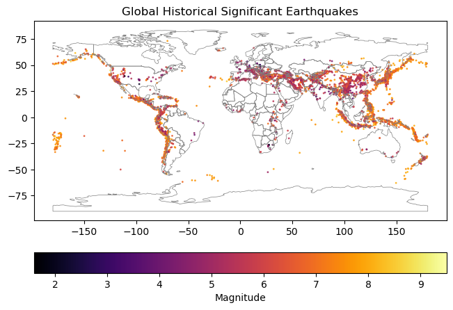
Vector example 3: NOAA’s Significant Earthquake Database

Read data

def load_and_prepare_earthquake_data():
    """
    Load and prepare global historical earthquake data from NOAA's API.
    Returns a GeoDataFrame of significant earthquakes.
    """
    # Use NOAA's official API endpoint for significant earthquakes
    base_url = "https://www.ngdc.noaa.gov/hazel/hazard-service/api/v1/earthquakes"
    
    # Get total number of pages from first request
    first_page = requests.get(base_url).json()
    total_pages = first_page['totalPages']
    
    # Initialize list to store all items
    all_items = []
    
    # Fetch all pages
    print(f"Fetching {total_pages} pages of earthquake data...")
    for page in range(total_pages):
        response = requests.get(f"{base_url}?page={page+1}").json()
        all_items.extend(response['items'])
    
    print(f"Total earthquakes fetched: {len(all_items)}")
    
    # Create DataFrame from all items
    df = pd.DataFrame(all_items)
    
    # Create GeoDataFrame from latitude and longitude
    gdf = gpd.GeoDataFrame(
        df, 
        geometry=gpd.points_from_xy(df.longitude, df.latitude),
        crs="EPSG:4326"  # WGS 84
    )
    
    # Filter for earthquakes with magnitude data
    gdf = gdf[gdf['eqMagnitude'].notna()]
    
    # Convert to Web Mercator for basemap compatibility
    #gdf = gdf.to_crs(epsg=3857)
    
    return gdf

earthquake_gdf = load_and_prepare_earthquake_data()

Fetching 33 pages of earthquake data...
Total earthquakes fetched: 6447

Preview data structure

earthquake_gdf

	id	year	locationName	latitude	longitude	eqMagnitude	damageAmountOrder	eqMagUnk	publish	country	...	area	eqMagMfa	damageMillionsDollars	missing	missingAmountOrder	missingTotal	missingAmountOrderTotal	damageMillionsDollarsTotal	eqMagMb	geometry
0	1	-2150	JORDAN: BAB-A-DARAA,AL-KARAK	31.100	35.500	7.3	3.0	7.3	True	JORDAN	...	NaN	NaN	NaN	NaN	NaN	NaN	NaN	NaN	NaN	POINT (35.5 31.1)
2	3	-2000	TURKMENISTAN: W	38.000	58.200	7.1	1.0	NaN	True	TURKMENISTAN	...	NaN	NaN	NaN	NaN	NaN	NaN	NaN	NaN	NaN	POINT (58.2 38)
5	12	-1250	ISRAEL: ARIHA (JERICHO)	32.000	35.500	6.5	3.0	6.5	True	ISRAEL	...	NaN	NaN	NaN	NaN	NaN	NaN	NaN	NaN	NaN	POINT (35.5 32)
6	13	-1050	JORDAN: SW: TIMNA COPPER MINES	29.600	35.000	6.2	3.0	6.2	True	JORDAN	...	NaN	NaN	NaN	NaN	NaN	NaN	NaN	NaN	NaN	POINT (35 29.6)
9	17	-479	GREECE: MACEDONIA	39.700	23.300	7.0	NaN	NaN	True	GREECE	...	NaN	NaN	NaN	NaN	NaN	NaN	NaN	NaN	NaN	POINT (23.3 39.7)
...	...	...	...	...	...	...	...	...	...	...	...	...	...	...	...	...	...	...	...	...	...
6441	10759	1570	OMAN: QALHAT	22.600	59.400	7.0	4.0	NaN	True	OMAN	...	NaN	NaN	NaN	NaN	NaN	NaN	NaN	NaN	NaN	POINT (59.4 22.6)
6442	10760	2024	TURKEY: ELAZIG AND MALATYA PROVINCES	38.309	38.826	6.0	2.0	NaN	True	TURKEY	...	NaN	NaN	NaN	NaN	NaN	NaN	NaN	NaN	NaN	POINT (38.826 38.309)
6443	10761	2024	CUBA: GRANMA, SANTIAGO DE CUBA	19.812	-77.039	6.8	3.0	NaN	True	CUBA	...	NaN	NaN	NaN	NaN	NaN	NaN	NaN	NaN	NaN	POINT (-77.039 19.812)
6444	10762	2024	CALIFORNIA: OFFSHORE CAPE MENDOCINO	40.374	-125.022	7.0	NaN	NaN	True	USA	...	CA	NaN	NaN	NaN	NaN	NaN	NaN	NaN	NaN	POINT (-125.022 40.374)
6445	10763	2024	VANUATU ISLANDS: EFATE, PORT VILA	-17.686	168.034	7.3	3.0	NaN	True	VANUATU	...	NaN	NaN	NaN	NaN	NaN	NaN	NaN	NaN	NaN	POINT (168.034 -17.686)

4672 rows × 50 columns

earthquake_gdf.shape

(4672, 50)

Visualize data

f, ax = plt.subplots(layout='compressed')

world_gdf.boundary.plot(ax=ax,color='grey',linewidth=0.5)

# Plot earthquakes
scatter = earthquake_gdf.plot(
    ax=ax,
    column='eqMagnitude',
    cmap='inferno',
    legend=True,
    legend_kwds={
        'label': 'Magnitude',
        'orientation': 'horizontal',
    },
    markersize=1,#earthquake_gdf['eqMagnitude'] * 1,  # Reduced size multiplier due to more points
    alpha=0.8
)

# # Add basemap
# ctx.add_basemap(
#     ax,
#     source=ctx.providers.Esri.WorldImagery
# )


ax.set_title('Global Historical Significant Earthquakes')

Text(0.5, 1.0, 'Global Historical Significant Earthquakes')

Raster example 1: Copernicus GLO-90 Digital Elevation Model

Read data

bbox = (-122.0, 46.7, -121.5, 47.0)

cop90_dem_da = easysnowdata.topography.get_copernicus_dem(bbox, resolution=90)

Preview data structure

cop90_dem_da

<xarray.DataArray 'data' (latitude: 361, longitude: 601)> Size: 868kB
dask.array<getitem, shape=(361, 601), dtype=float32, chunksize=(361, 601), chunktype=numpy.ndarray>
Coordinates:
  * latitude     (latitude) float64 3kB 47.0 47.0 47.0 47.0 ... 46.7 46.7 46.7
  * longitude    (longitude) float64 5kB -122.0 -122.0 -122.0 ... -121.5 -121.5
    spatial_ref  int32 4B 4326
    time         datetime64[ns] 8B 2021-04-22

xarray.DataArray

'data'

• latitude: 361
• longitude: 601

• dask.array<chunksize=(361, 601), meta=np.ndarray>

  Array Chunk Bytes 847.50 kiB 847.50 kiB Shape (361, 601) (361, 601) Dask graph 1 chunks in 4 graph layers Data type float32 numpy.ndarray

• Coordinates: (4)
  • latitude
    (latitude)
    float64
    47.0 47.0 47.0 ... 46.7 46.7 46.7

    units :

    degrees_north

    resolution :

    -0.0008333333333333334

    crs :

    EPSG:4326

    array([47.      , 46.999167, 46.998333, ..., 46.701667, 46.700833, 46.7     ])

  • longitude
    (longitude)
    float64
    -122.0 -122.0 ... -121.5 -121.5

    units :

    degrees_east

    resolution :

    0.0008333333333333334

    crs :

    EPSG:4326

    array([-122.      , -121.999167, -121.998333, ..., -121.501667, -121.500833,
           -121.5     ])

  • spatial_ref
    ()
    int32
    4326

    spatial_ref :

    GEOGCRS["WGS 84",ENSEMBLE["World Geodetic System 1984 ensemble",MEMBER["World Geodetic System 1984 (Transit)"],MEMBER["World Geodetic System 1984 (G730)"],MEMBER["World Geodetic System 1984 (G873)"],MEMBER["World Geodetic System 1984 (G1150)"],MEMBER["World Geodetic System 1984 (G1674)"],MEMBER["World Geodetic System 1984 (G1762)"],MEMBER["World Geodetic System 1984 (G2139)"],MEMBER["World Geodetic System 1984 (G2296)"],ELLIPSOID["WGS 84",6378137,298.257223563,LENGTHUNIT["metre",1]],ENSEMBLEACCURACY[2.0]],PRIMEM["Greenwich",0,ANGLEUNIT["degree",0.0174532925199433]],CS[ellipsoidal,2],AXIS["geodetic latitude (Lat)",north,ORDER[1],ANGLEUNIT["degree",0.0174532925199433]],AXIS["geodetic longitude (Lon)",east,ORDER[2],ANGLEUNIT["degree",0.0174532925199433]],USAGE[SCOPE["Horizontal component of 3D system."],AREA["World."],BBOX[-90,-180,90,180]],ID["EPSG",4326]]

    crs_wkt :

    GEOGCRS["WGS 84",ENSEMBLE["World Geodetic System 1984 ensemble",MEMBER["World Geodetic System 1984 (Transit)"],MEMBER["World Geodetic System 1984 (G730)"],MEMBER["World Geodetic System 1984 (G873)"],MEMBER["World Geodetic System 1984 (G1150)"],MEMBER["World Geodetic System 1984 (G1674)"],MEMBER["World Geodetic System 1984 (G1762)"],MEMBER["World Geodetic System 1984 (G2139)"],MEMBER["World Geodetic System 1984 (G2296)"],ELLIPSOID["WGS 84",6378137,298.257223563,LENGTHUNIT["metre",1]],ENSEMBLEACCURACY[2.0]],PRIMEM["Greenwich",0,ANGLEUNIT["degree",0.0174532925199433]],CS[ellipsoidal,2],AXIS["geodetic latitude (Lat)",north,ORDER[1],ANGLEUNIT["degree",0.0174532925199433]],AXIS["geodetic longitude (Lon)",east,ORDER[2],ANGLEUNIT["degree",0.0174532925199433]],USAGE[SCOPE["Horizontal component of 3D system."],AREA["World."],BBOX[-90,-180,90,180]],ID["EPSG",4326]]

    semi_major_axis :

    6378137.0

    semi_minor_axis :

    6356752.314245179

    inverse_flattening :

    298.257223563

    reference_ellipsoid_name :

    WGS 84

    longitude_of_prime_meridian :

    0.0

    prime_meridian_name :

    Greenwich

    geographic_crs_name :

    WGS 84

    horizontal_datum_name :

    World Geodetic System 1984 ensemble

    grid_mapping_name :

    latitude_longitude

    GeoTransform :

    -122.000416666666680498565256 0.000833333333333333386821 0 47.000416666666673393137899 0 -0.000833333333333333386821

    array(4326, dtype=int32)

  • time
    ()
    datetime64[ns]
    2021-04-22

    array('2021-04-22T00:00:00.000000000', dtype='datetime64[ns]')

• Indexes: (2)
  • latitude
    PandasIndex

    PandasIndex(Index([ 47.00000000000001, 46.999166666666675,  46.99833333333334,
            46.99750000000001,  46.99666666666668,  46.99583333333334,
           46.995000000000005,  46.99416666666667,  46.99333333333334,
            46.99250000000001,
           ...
            46.70750000000001,  46.70666666666667,  46.70583333333334,
           46.705000000000005,  46.70416666666667,  46.70333333333334,
            46.70250000000001, 46.701666666666675,  46.70083333333334,
            46.70000000000001],
          dtype='float64', name='latitude', length=361))

  • longitude
    PandasIndex

    PandasIndex(Index([-122.00000000000001, -121.99916666666668, -121.99833333333335,
           -121.99750000000002, -121.99666666666668, -121.99583333333335,
           -121.99500000000002, -121.99416666666669, -121.99333333333335,
           -121.99250000000002,
           ...
           -121.50750000000001, -121.50666666666667, -121.50583333333334,
           -121.50500000000001, -121.50416666666668, -121.50333333333334,
           -121.50250000000001, -121.50166666666668, -121.50083333333335,
           -121.50000000000001],
          dtype='float64', name='longitude', length=601))

• Attributes: (0)

cop90_dem_da.values

array([[ 499.2021 ,  496.54   ,  495.75162, ..., 1218.6013 , 1234.3867 ,
        1233.8529 ],
       [ 508.11026,  508.29654,  507.0695 , ..., 1155.2106 , 1165.3165 ,
        1167.0106 ],
       [ 519.83374,  517.6379 ,  515.73   , ..., 1095.627  , 1106.0608 ,
        1106.6742 ],
       ...,
       [ 984.7717 ,  955.91187,  929.96   , ..., 1208.51   , 1210.0714 ,
        1209.9208 ],
       [ 950.2026 ,  925.1188 ,  901.5398 , ..., 1207.794  , 1216.0377 ,
        1216.38   ],
       [ 915.3658 ,  893.26587,  872.855  , ..., 1206.2902 , 1217.8804 ,
        1224.1011 ]], dtype=float32)

np.shape(cop90_dem_da.values)

(361, 601)

Visualize data

f,ax=plt.subplots(layout='compressed')
cop90_dem_da.plot(ax=ax,cmap='terrain')
ax.set_title('Copernicus GLO-90 DEM')

Text(0.5, 1.0, 'Copernicus GLO-90 DEM')

Raster example 2: ESA WorldCover 2021

Read data

worldcover_da = easysnowdata.remote_sensing.get_esa_worldcover(bbox)

Preview data structure

worldcover_da

<xarray.DataArray 'map' (latitude: 3600, longitude: 6000)> Size: 22MB
dask.array<getitem, shape=(3600, 6000), dtype=uint8, chunksize=(3600, 6000), chunktype=numpy.ndarray>
Coordinates:
  * latitude     (latitude) float64 29kB 47.0 47.0 47.0 47.0 ... 46.7 46.7 46.7
  * longitude    (longitude) float64 48kB -122.0 -122.0 -122.0 ... -121.5 -121.5
    spatial_ref  int32 4B 4326
    time         datetime64[ns] 8B 2021-01-01
Attributes:
    nodata:         0
    class_info:     {10: {'name': 'Tree cover', 'color': '#006400'}, 20: {'na...
    cmap:           <matplotlib.colors.ListedColormap object at 0x7ac749e91490>
    data_citation:  Zanaga, D., Van De Kerchove, R., De Keersmaecker, W., Sou...
    example_plot:   <function get_esa_worldcover.<locals>.plot_classes at 0x7...

xarray.DataArray

'map'

• latitude: 3600
• longitude: 6000

• dask.array<chunksize=(3600, 6000), meta=np.ndarray>

  Array Chunk Bytes 20.60 MiB 20.60 MiB Shape (3600, 6000) (3600, 6000) Dask graph 1 chunks in 5 graph layers Data type uint8 numpy.ndarray

• Coordinates: (4)
  • latitude
    (latitude)
    float64
    47.0 47.0 47.0 ... 46.7 46.7 46.7

    units :

    degrees_north

    resolution :

    -8.333333333333333e-05

    crs :

    EPSG:4326

    array([46.999958, 46.999875, 46.999792, ..., 46.700208, 46.700125, 46.700042])

  • longitude
    (longitude)
    float64
    -122.0 -122.0 ... -121.5 -121.5

    units :

    degrees_east

    resolution :

    8.333333333333333e-05

    crs :

    EPSG:4326

    array([-121.999958, -121.999875, -121.999792, ..., -121.500208, -121.500125,
           -121.500042])

  • spatial_ref
    ()
    int32
    4326

    spatial_ref :

    GEOGCRS["WGS 84",ENSEMBLE["World Geodetic System 1984 ensemble",MEMBER["World Geodetic System 1984 (Transit)"],MEMBER["World Geodetic System 1984 (G730)"],MEMBER["World Geodetic System 1984 (G873)"],MEMBER["World Geodetic System 1984 (G1150)"],MEMBER["World Geodetic System 1984 (G1674)"],MEMBER["World Geodetic System 1984 (G1762)"],MEMBER["World Geodetic System 1984 (G2139)"],MEMBER["World Geodetic System 1984 (G2296)"],ELLIPSOID["WGS 84",6378137,298.257223563,LENGTHUNIT["metre",1]],ENSEMBLEACCURACY[2.0]],PRIMEM["Greenwich",0,ANGLEUNIT["degree",0.0174532925199433]],CS[ellipsoidal,2],AXIS["geodetic latitude (Lat)",north,ORDER[1],ANGLEUNIT["degree",0.0174532925199433]],AXIS["geodetic longitude (Lon)",east,ORDER[2],ANGLEUNIT["degree",0.0174532925199433]],USAGE[SCOPE["Horizontal component of 3D system."],AREA["World."],BBOX[-90,-180,90,180]],ID["EPSG",4326]]

    crs_wkt :

    GEOGCRS["WGS 84",ENSEMBLE["World Geodetic System 1984 ensemble",MEMBER["World Geodetic System 1984 (Transit)"],MEMBER["World Geodetic System 1984 (G730)"],MEMBER["World Geodetic System 1984 (G873)"],MEMBER["World Geodetic System 1984 (G1150)"],MEMBER["World Geodetic System 1984 (G1674)"],MEMBER["World Geodetic System 1984 (G1762)"],MEMBER["World Geodetic System 1984 (G2139)"],MEMBER["World Geodetic System 1984 (G2296)"],ELLIPSOID["WGS 84",6378137,298.257223563,LENGTHUNIT["metre",1]],ENSEMBLEACCURACY[2.0]],PRIMEM["Greenwich",0,ANGLEUNIT["degree",0.0174532925199433]],CS[ellipsoidal,2],AXIS["geodetic latitude (Lat)",north,ORDER[1],ANGLEUNIT["degree",0.0174532925199433]],AXIS["geodetic longitude (Lon)",east,ORDER[2],ANGLEUNIT["degree",0.0174532925199433]],USAGE[SCOPE["Horizontal component of 3D system."],AREA["World."],BBOX[-90,-180,90,180]],ID["EPSG",4326]]

    semi_major_axis :

    6378137.0

    semi_minor_axis :

    6356752.314245179

    inverse_flattening :

    298.257223563

    reference_ellipsoid_name :

    WGS 84

    longitude_of_prime_meridian :

    0.0

    prime_meridian_name :

    Greenwich

    geographic_crs_name :

    WGS 84

    horizontal_datum_name :

    World Geodetic System 1984 ensemble

    grid_mapping_name :

    latitude_longitude

    GeoTransform :

    -122 0.000083333333333333330551 0 46.999999999999992894572642 0 -0.000083333333333333330551

    array(4326, dtype=int32)

  • time
    ()
    datetime64[ns]
    2021-01-01

    array('2021-01-01T00:00:00.000000000', dtype='datetime64[ns]')

• Indexes: (2)
  • latitude
    PandasIndex

    PandasIndex(Index([46.999958333333325,  46.99987499999999,  46.99979166666666,
           46.999708333333324, 46.999624999999995,  46.99954166666666,
            46.99945833333332,  46.99937499999999,  46.99929166666666,
            46.99920833333333,
           ...
            46.70079166666666, 46.700708333333324,  46.70062499999999,
            46.70054166666666,  46.70045833333332, 46.700374999999994,
            46.70029166666666,  46.70020833333332,  46.70012499999999,
            46.70004166666666],
          dtype='float64', name='latitude', length=3600))

  • longitude
    PandasIndex

    PandasIndex(Index([-121.99995833333334,         -121.999875, -121.99979166666667,
           -121.99970833333334, -121.99962500000001, -121.99954166666667,
           -121.99945833333334,         -121.999375, -121.99929166666668,
           -121.99920833333334,
           ...
           -121.50079166666667, -121.50070833333334,         -121.500625,
           -121.50054166666668, -121.50045833333334,         -121.500375,
           -121.50029166666667, -121.50020833333333, -121.50012500000001,
           -121.50004166666668],
          dtype='float64', name='longitude', length=6000))

• Attributes: (5)

  nodata :

  0

  class_info :

  {10: {'name': 'Tree cover', 'color': '#006400'}, 20: {'name': 'Shrubland', 'color': '#FFBB22'}, 30: {'name': 'Grassland', 'color': '#FFFF4C'}, 40: {'name': 'Cropland', 'color': '#F096FF'}, 50: {'name': 'Built-up', 'color': '#FA0000'}, 60: {'name': 'Bare / sparse vegetation', 'color': '#B4B4B4'}, 70: {'name': 'Snow and ice', 'color': '#F0F0F0'}, 80: {'name': 'Permanent water bodies', 'color': '#0064C8'}, 90: {'name': 'Herbaceous wetland', 'color': '#0096A0'}, 95: {'name': 'Mangroves', 'color': '#00CF75'}, 100: {'name': 'Moss and lichen', 'color': '#FAE6A0'}}

  cmap :

  <matplotlib.colors.ListedColormap object at 0x7ac749e91490>

  data_citation :

  Zanaga, D., Van De Kerchove, R., De Keersmaecker, W., Souverijns, N., Brockmann, C., Quast, R., Wevers, J., Grosu, A., Paccini, A., Vergnaud, S., Cartus, O., Santoro, M., Fritz, S., Georgieva, I., Lesiv, M., Carter, S., Herold, M., Li, Linlin, Tsendbazar, N.E., Ramoino, F., Arino, O. (2021). ESA WorldCover 10 m 2020 v100. doi:10.5281/zenodo.5571936.

  example_plot :

  <function get_esa_worldcover.<locals>.plot_classes at 0x7ac74970f880>

worldcover_da.values

array([[10, 10, 10, ..., 10, 10, 10],
       [10, 10, 10, ..., 10, 10, 10],
       [10, 10, 10, ..., 10, 10, 10],
       ...,
       [10, 10, 10, ..., 10, 10, 10],
       [10, 10, 10, ..., 10, 10, 10],
       [10, 10, 10, ..., 10, 10, 10]], dtype=uint8)

np.shape(worldcover_da.values)

(3600, 6000)

Visualize data

f, ax = worldcover_da.attrs['example_plot'](worldcover_da)

Raster example 3: Sentinel-2 RGB image

Read data

def norm(a, perc_lim=(2, 98), clip=True, verbose=False):
    #Simple approach using actual min and max values
    #amin, amax = (a.min(), a.max())
    #Check if we're using masked array or np.nan
    if np.ma.isMaskedArray(a):
        amin, amax = np.percentile(a.compressed(), perc_lim)
    else:
        amin, amax = np.nanpercentile(a, perc_lim)
    out = ((a - amin)/(amax - amin))
    #This will "clip" normalized values <0 to 0 and >1 to 1
    if clip:
        out = out.clip(0,1)
    if verbose:
        print("Input range: ({}, {})".format(a.min(), a.max()))
        print(f"Percentile range {perc_lim}: ({amin}, {amax})")
        print("Output range: ({}, {})".format(out.min(), out.max()))
    return out
    
catalog = pystac_client.Client.open(
    "https://planetarycomputer.microsoft.com/api/stac/v1",
    modifier=planetary_computer.sign_inplace,
)

search = catalog.search(
    collections=["sentinel-2-l2a"],
    bbox=bbox,
    datetime=("2022-07-31", "2022-07-31"),
)
red_fn = search.item_collection()[3].assets['B04'].href
green_fn = search.item_collection()[3].assets['B03'].href
blue_fn = search.item_collection()[3].assets['B02'].href

red_src = rio.open(red_fn)
window = rio.windows.Window(8000, 0, 3*1024, 2*1024)
window_bounds = rio.windows.bounds(window, red_src.transform)
window_extent = [window_bounds[0], window_bounds[2], window_bounds[1], window_bounds[3]]

r = rio.open(red_fn).read(1,window=window)
g = rio.open(green_fn).read(1,window=window)
b = rio.open(blue_fn).read(1,window=window)

perc = (0, 90)

r_norm = norm(r, perc)
g_norm = norm(g, perc)
b_norm = norm(b, perc)


rgb = np.dstack([r_norm,g_norm,b_norm])

Preview data structure

rgb

array([[[0.25661157, 0.26189128, 0.2309719 ],
        [0.32203857, 0.28765572, 0.27078454],
        [0.29201102, 0.28015289, 0.26478337],
        ...,
        [0.16143251, 0.19252548, 0.17300937],
        [0.16212121, 0.18530578, 0.17740047],
        [0.16639118, 0.18587203, 0.17227752]],

       [[0.23168044, 0.22989807, 0.21574941],
        [0.29173554, 0.26642129, 0.25263466],
        [0.28732782, 0.26882786, 0.26009953],
        ...,
        [0.1584022 , 0.18162514, 0.17242389],
        [0.15275482, 0.16208947, 0.16569087],
        [0.1523416 , 0.16605323, 0.16583724]],

       [[0.184573  , 0.20385051, 0.18881733],
        [0.21184573, 0.21191959, 0.19672131],
        [0.21983471, 0.22197055, 0.20769906],
        ...,
        [0.15055096, 0.15812571, 0.16129977],
        [0.15013774, 0.16718573, 0.16144614],
        [0.15275482, 0.17468856, 0.16671546]],

       ...,

       [[0.16363636, 0.1867214 , 0.17637588],
        [0.1607438 , 0.1817667 , 0.17652225],
        [0.15922865, 0.18035108, 0.17476581],
        ...,
        [0.15247934, 0.17780294, 0.16378806],
        [0.15922865, 0.17709513, 0.1684719 ],
        [0.15716253, 0.17412231, 0.16598361]],

       [[0.16143251, 0.1882786 , 0.1743267 ],
        [0.15936639, 0.18105889, 0.16964286],
        [0.15426997, 0.17539638, 0.17110656],
        ...,
        [0.1577135 , 0.18884485, 0.16686183],
        [0.16143251, 0.18360702, 0.16978923],
        [0.15716253, 0.17313137, 0.16598361]],

       [[0.15964187, 0.18148358, 0.17505855],
        [0.15730028, 0.17667044, 0.17052108],
        [0.15495868, 0.17921857, 0.17096019],
        ...,
        [0.15523416, 0.18374858, 0.16759368],
        [0.16033058, 0.18403171, 0.16276347],
        [0.16859504, 0.19266704, 0.17271663]]])

np.shape(rgb)

(2048, 2980, 3)

Visualize data

f, axs = plt.subplots(2,2, layout='compressed',sharex=True,sharey=True)
axs[0,0].imshow(rgb[:,:,0], cmap='Reds',extent=window_extent)
axs[0,1].imshow(rgb[:,:,1], cmap='Greens',extent=window_extent)
axs[1,0].imshow(rgb[:,:,2], cmap='Blues',extent=window_extent)
axs[1,1].imshow(rgb,extent=window_extent)

axs[0,0].set_title('Red band')
axs[0,1].set_title('Green band')
axs[1,0].set_title('Blue band')
axs[1,1].set_title('RGB image')

for ax in axs.flat:
    ax.set_aspect('equal')

nDarray example 1: Sentinel-2 image stack

Read data

bbox = (-122.0, 46.7, -121.5, 47.0)

s2 = easysnowdata.remote_sensing.Sentinel2(
    bbox_input=bbox,
    start_date="2022-07-21",
    end_date="2022-07-31",
    resolution=80,
)

Data searched. Access the returned seach with the .search attribute.
Data retrieved. Access with the .data attribute. Data CRS: WGS 84 / UTM zone 10N.
Nodata values removed from the data. In doing so, all bands converted to float32. To turn this behavior off, set remove_nodata=False.
Data acquired after January 25th, 2022 harmonized to old baseline. To override this behavior, set harmonize_to_old=False.
Data scaled to float reflectance. To turn this behavior off, set scale_data=False.
Metadata retrieved. Access with the .metadata attribute.

Preview data structure

s2.data # click through data variables to explore the structure!

<xarray.Dataset> Size: 66MB
Dimensions:      (time: 5, y: 426, x: 484)
Coordinates:
  * y            (y) float64 3kB 5.206e+06 5.206e+06 ... 5.172e+06 5.172e+06
  * x            (x) float64 4kB 5.76e+05 5.761e+05 ... 6.146e+05 6.147e+05
    spatial_ref  int32 4B 32610
  * time         (time) datetime64[ns] 40B 2022-07-21T18:59:19.024000 ... 202...
Data variables: (12/16)
    coastal      (time, y, x) float32 4MB dask.array<chunksize=(1, 426, 484), meta=np.ndarray>
    blue         (time, y, x) float32 4MB dask.array<chunksize=(1, 426, 484), meta=np.ndarray>
    green        (time, y, x) float32 4MB dask.array<chunksize=(1, 426, 484), meta=np.ndarray>
    red          (time, y, x) float32 4MB dask.array<chunksize=(1, 426, 484), meta=np.ndarray>
    rededge      (time, y, x) float32 4MB dask.array<chunksize=(1, 426, 484), meta=np.ndarray>
    rededge2     (time, y, x) float32 4MB dask.array<chunksize=(1, 426, 484), meta=np.ndarray>
    ...           ...
    swir16       (time, y, x) float32 4MB dask.array<chunksize=(1, 426, 484), meta=np.ndarray>
    swir22       (time, y, x) float32 4MB dask.array<chunksize=(1, 426, 484), meta=np.ndarray>
    aot          (time, y, x) float32 4MB dask.array<chunksize=(1, 426, 484), meta=np.ndarray>
    scl          (time, y, x) float32 4MB dask.array<chunksize=(1, 426, 484), meta=np.ndarray>
    wvp          (time, y, x) float32 4MB dask.array<chunksize=(1, 426, 484), meta=np.ndarray>
    visual       (time, y, x) float32 4MB dask.array<chunksize=(1, 426, 484), meta=np.ndarray>
Attributes:
    band_info:       {'B01': {'name': 'coastal', 'description': 'Coastal aero...
    scl_class_info:  {0: {'name': 'No Data (Missing data)', 'color': '#000000...

xarray.Dataset

• Dimensions:
  • time: 5
  • y: 426
  • x: 484
• Coordinates: (4)
  • y
    (y)
    float64
    5.206e+06 5.206e+06 ... 5.172e+06

    units :

    metre

    resolution :

    -80.0

    crs :

    EPSG:32610

    array([5206280., 5206200., 5206120., ..., 5172440., 5172360., 5172280.])

  • x
    (x)
    float64
    5.76e+05 5.761e+05 ... 6.147e+05

    units :

    metre

    resolution :

    80.0

    crs :

    EPSG:32610

    array([576040., 576120., 576200., ..., 614520., 614600., 614680.])

  • spatial_ref
    ()
    int32
    32610

    spatial_ref :

    PROJCRS["WGS 84 / UTM zone 10N",BASEGEOGCRS["WGS 84",ENSEMBLE["World Geodetic System 1984 ensemble",MEMBER["World Geodetic System 1984 (Transit)"],MEMBER["World Geodetic System 1984 (G730)"],MEMBER["World Geodetic System 1984 (G873)"],MEMBER["World Geodetic System 1984 (G1150)"],MEMBER["World Geodetic System 1984 (G1674)"],MEMBER["World Geodetic System 1984 (G1762)"],MEMBER["World Geodetic System 1984 (G2139)"],MEMBER["World Geodetic System 1984 (G2296)"],ELLIPSOID["WGS 84",6378137,298.257223563,LENGTHUNIT["metre",1]],ENSEMBLEACCURACY[2.0]],PRIMEM["Greenwich",0,ANGLEUNIT["degree",0.0174532925199433]],ID["EPSG",4326]],CONVERSION["UTM zone 10N",METHOD["Transverse Mercator",ID["EPSG",9807]],PARAMETER["Latitude of natural origin",0,ANGLEUNIT["degree",0.0174532925199433],ID["EPSG",8801]],PARAMETER["Longitude of natural origin",-123,ANGLEUNIT["degree",0.0174532925199433],ID["EPSG",8802]],PARAMETER["Scale factor at natural origin",0.9996,SCALEUNIT["unity",1],ID["EPSG",8805]],PARAMETER["False easting",500000,LENGTHUNIT["metre",1],ID["EPSG",8806]],PARAMETER["False northing",0,LENGTHUNIT["metre",1],ID["EPSG",8807]]],CS[Cartesian,2],AXIS["(E)",east,ORDER[1],LENGTHUNIT["metre",1]],AXIS["(N)",north,ORDER[2],LENGTHUNIT["metre",1]],USAGE[SCOPE["Navigation and medium accuracy spatial referencing."],AREA["Between 126°W and 120°W, northern hemisphere between equator and 84°N, onshore and offshore. Canada - British Columbia (BC); Northwest Territories (NWT); Nunavut; Yukon. United States (USA) - Alaska (AK)."],BBOX[0,-126,84,-120]],ID["EPSG",32610]]

    crs_wkt :

    PROJCRS["WGS 84 / UTM zone 10N",BASEGEOGCRS["WGS 84",ENSEMBLE["World Geodetic System 1984 ensemble",MEMBER["World Geodetic System 1984 (Transit)"],MEMBER["World Geodetic System 1984 (G730)"],MEMBER["World Geodetic System 1984 (G873)"],MEMBER["World Geodetic System 1984 (G1150)"],MEMBER["World Geodetic System 1984 (G1674)"],MEMBER["World Geodetic System 1984 (G1762)"],MEMBER["World Geodetic System 1984 (G2139)"],MEMBER["World Geodetic System 1984 (G2296)"],ELLIPSOID["WGS 84",6378137,298.257223563,LENGTHUNIT["metre",1]],ENSEMBLEACCURACY[2.0]],PRIMEM["Greenwich",0,ANGLEUNIT["degree",0.0174532925199433]],ID["EPSG",4326]],CONVERSION["UTM zone 10N",METHOD["Transverse Mercator",ID["EPSG",9807]],PARAMETER["Latitude of natural origin",0,ANGLEUNIT["degree",0.0174532925199433],ID["EPSG",8801]],PARAMETER["Longitude of natural origin",-123,ANGLEUNIT["degree",0.0174532925199433],ID["EPSG",8802]],PARAMETER["Scale factor at natural origin",0.9996,SCALEUNIT["unity",1],ID["EPSG",8805]],PARAMETER["False easting",500000,LENGTHUNIT["metre",1],ID["EPSG",8806]],PARAMETER["False northing",0,LENGTHUNIT["metre",1],ID["EPSG",8807]]],CS[Cartesian,2],AXIS["(E)",east,ORDER[1],LENGTHUNIT["metre",1]],AXIS["(N)",north,ORDER[2],LENGTHUNIT["metre",1]],USAGE[SCOPE["Navigation and medium accuracy spatial referencing."],AREA["Between 126°W and 120°W, northern hemisphere between equator and 84°N, onshore and offshore. Canada - British Columbia (BC); Northwest Territories (NWT); Nunavut; Yukon. United States (USA) - Alaska (AK)."],BBOX[0,-126,84,-120]],ID["EPSG",32610]]

    semi_major_axis :

    6378137.0

    semi_minor_axis :

    6356752.314245179

    inverse_flattening :

    298.257223563

    reference_ellipsoid_name :

    WGS 84

    longitude_of_prime_meridian :

    0.0

    prime_meridian_name :

    Greenwich

    geographic_crs_name :

    WGS 84

    horizontal_datum_name :

    World Geodetic System 1984 ensemble

    projected_crs_name :

    WGS 84 / UTM zone 10N

    grid_mapping_name :

    transverse_mercator

    latitude_of_projection_origin :

    0.0

    longitude_of_central_meridian :

    -123.0

    false_easting :

    500000.0

    false_northing :

    0.0

    scale_factor_at_central_meridian :

    0.9996

    GeoTransform :

    576000 80 0 5206320 0 -80

    array(32610, dtype=int32)

  • time
    (time)
    datetime64[ns]
    2022-07-21T18:59:19.024000 ... 2...

    array(['2022-07-21T18:59:19.024000000', '2022-07-24T19:09:19.024000000',
           '2022-07-26T18:59:31.024000000', '2022-07-29T19:09:21.024000000',
           '2022-07-31T18:59:19.024000000'], dtype='datetime64[ns]')

• Data variables: (16)
  • coastal
    (time, y, x)
    float32
    dask.array<chunksize=(1, 426, 484), meta=np.ndarray>

    nodata :

    0

    Array Chunk Bytes 3.93 MiB 805.41 kiB Shape (5, 426, 484) (1, 426, 484) Dask graph 5 chunks in 9 graph layers Data type float32 numpy.ndarray

  • blue
    (time, y, x)
    float32
    dask.array<chunksize=(1, 426, 484), meta=np.ndarray>

    nodata :

    0

    Array Chunk Bytes 3.93 MiB 805.41 kiB Shape (5, 426, 484) (1, 426, 484) Dask graph 5 chunks in 9 graph layers Data type float32 numpy.ndarray

  • green
    (time, y, x)
    float32
    dask.array<chunksize=(1, 426, 484), meta=np.ndarray>

    nodata :

    0

    Array Chunk Bytes 3.93 MiB 805.41 kiB Shape (5, 426, 484) (1, 426, 484) Dask graph 5 chunks in 9 graph layers Data type float32 numpy.ndarray

  • red
    (time, y, x)
    float32
    dask.array<chunksize=(1, 426, 484), meta=np.ndarray>

    nodata :

    0

    Array Chunk Bytes 3.93 MiB 805.41 kiB Shape (5, 426, 484) (1, 426, 484) Dask graph 5 chunks in 9 graph layers Data type float32 numpy.ndarray

  • rededge
    (time, y, x)
    float32
    dask.array<chunksize=(1, 426, 484), meta=np.ndarray>

    nodata :

    0

    Array Chunk Bytes 3.93 MiB 805.41 kiB Shape (5, 426, 484) (1, 426, 484) Dask graph 5 chunks in 9 graph layers Data type float32 numpy.ndarray

  • rededge2
    (time, y, x)
    float32
    dask.array<chunksize=(1, 426, 484), meta=np.ndarray>

    nodata :

    0

    Array Chunk Bytes 3.93 MiB 805.41 kiB Shape (5, 426, 484) (1, 426, 484) Dask graph 5 chunks in 9 graph layers Data type float32 numpy.ndarray

  • rededge3
    (time, y, x)
    float32
    dask.array<chunksize=(1, 426, 484), meta=np.ndarray>

    nodata :

    0

    Array Chunk Bytes 3.93 MiB 805.41 kiB Shape (5, 426, 484) (1, 426, 484) Dask graph 5 chunks in 9 graph layers Data type float32 numpy.ndarray

  • nir
    (time, y, x)
    float32
    dask.array<chunksize=(1, 426, 484), meta=np.ndarray>

    nodata :

    0

    Array Chunk Bytes 3.93 MiB 805.41 kiB Shape (5, 426, 484) (1, 426, 484) Dask graph 5 chunks in 9 graph layers Data type float32 numpy.ndarray

  • nir08
    (time, y, x)
    float32
    dask.array<chunksize=(1, 426, 484), meta=np.ndarray>

    nodata :

    0

    Array Chunk Bytes 3.93 MiB 805.41 kiB Shape (5, 426, 484) (1, 426, 484) Dask graph 5 chunks in 9 graph layers Data type float32 numpy.ndarray

  • nir09
    (time, y, x)
    float32
    dask.array<chunksize=(1, 426, 484), meta=np.ndarray>

    nodata :

    0

    Array Chunk Bytes 3.93 MiB 805.41 kiB Shape (5, 426, 484) (1, 426, 484) Dask graph 5 chunks in 9 graph layers Data type float32 numpy.ndarray

  • swir16
    (time, y, x)
    float32
    dask.array<chunksize=(1, 426, 484), meta=np.ndarray>

    nodata :

    0

    Array Chunk Bytes 3.93 MiB 805.41 kiB Shape (5, 426, 484) (1, 426, 484) Dask graph 5 chunks in 9 graph layers Data type float32 numpy.ndarray

  • swir22
    (time, y, x)
    float32
    dask.array<chunksize=(1, 426, 484), meta=np.ndarray>

    nodata :

    0

    Array Chunk Bytes 3.93 MiB 805.41 kiB Shape (5, 426, 484) (1, 426, 484) Dask graph 5 chunks in 9 graph layers Data type float32 numpy.ndarray

  • aot
    (time, y, x)
    float32
    dask.array<chunksize=(1, 426, 484), meta=np.ndarray>

    nodata :

    0

    Array Chunk Bytes 3.93 MiB 805.41 kiB Shape (5, 426, 484) (1, 426, 484) Dask graph 5 chunks in 7 graph layers Data type float32 numpy.ndarray

  • scl
    (time, y, x)
    float32
    dask.array<chunksize=(1, 426, 484), meta=np.ndarray>

    nodata :

    0

    scl_class_info :

    {0: {'name': 'No Data (Missing data)', 'color': '#000000'}, 1: {'name': 'Saturated or defective pixel', 'color': '#ff0000'}, 2: {'name': 'Topographic casted shadows', 'color': '#2f2f2f'}, 3: {'name': 'Cloud shadows', 'color': '#643200'}, 4: {'name': 'Vegetation', 'color': '#00a000'}, 5: {'name': 'Not-vegetated', 'color': '#ffe65a'}, 6: {'name': 'Water', 'color': '#0000ff'}, 7: {'name': 'Unclassified', 'color': '#808080'}, 8: {'name': 'Cloud medium probability', 'color': '#c0c0c0'}, 9: {'name': 'Cloud high probability', 'color': '#ffffff'}, 10: {'name': 'Thin cirrus', 'color': '#64c8ff'}, 11: {'name': 'Snow or ice', 'color': '#ff96ff'}}

    example_plot :

    <bound method Sentinel2.plot_scl of <easysnowdata.remote_sensing.Sentinel2 object at 0x7ac749d95b80>>

    class_info :

    {0: {'name': 'No Data (Missing data)', 'color': '#000000'}, 1: {'name': 'Saturated or defective pixel', 'color': '#ff0000'}, 2: {'name': 'Topographic casted shadows', 'color': '#2f2f2f'}, 3: {'name': 'Cloud shadows', 'color': '#643200'}, 4: {'name': 'Vegetation', 'color': '#00a000'}, 5: {'name': 'Not-vegetated', 'color': '#ffe65a'}, 6: {'name': 'Water', 'color': '#0000ff'}, 7: {'name': 'Unclassified', 'color': '#808080'}, 8: {'name': 'Cloud medium probability', 'color': '#c0c0c0'}, 9: {'name': 'Cloud high probability', 'color': '#ffffff'}, 10: {'name': 'Thin cirrus', 'color': '#64c8ff'}, 11: {'name': 'Snow or ice', 'color': '#ff96ff'}}

    cmap :

    <matplotlib.colors.ListedColormap object at 0x7ac74958de80>

    Array Chunk Bytes 3.93 MiB 805.41 kiB Shape (5, 426, 484) (1, 426, 484) Dask graph 5 chunks in 7 graph layers Data type float32 numpy.ndarray

  • wvp
    (time, y, x)
    float32
    dask.array<chunksize=(1, 426, 484), meta=np.ndarray>

    nodata :

    0

    Array Chunk Bytes 3.93 MiB 805.41 kiB Shape (5, 426, 484) (1, 426, 484) Dask graph 5 chunks in 7 graph layers Data type float32 numpy.ndarray

  • visual
    (time, y, x)
    float32
    dask.array<chunksize=(1, 426, 484), meta=np.ndarray>

    nodata :

    0

    Array Chunk Bytes 3.93 MiB 805.41 kiB Shape (5, 426, 484) (1, 426, 484) Dask graph 5 chunks in 7 graph layers Data type float32 numpy.ndarray

• Indexes: (3)
  • y
    PandasIndex

    PandasIndex(Index([5206280.0, 5206200.0, 5206120.0, 5206040.0, 5205960.0, 5205880.0,
           5205800.0, 5205720.0, 5205640.0, 5205560.0,
           ...
           5173000.0, 5172920.0, 5172840.0, 5172760.0, 5172680.0, 5172600.0,
           5172520.0, 5172440.0, 5172360.0, 5172280.0],
          dtype='float64', name='y', length=426))

  • x
    PandasIndex

    PandasIndex(Index([576040.0, 576120.0, 576200.0, 576280.0, 576360.0, 576440.0, 576520.0,
           576600.0, 576680.0, 576760.0,
           ...
           613960.0, 614040.0, 614120.0, 614200.0, 614280.0, 614360.0, 614440.0,
           614520.0, 614600.0, 614680.0],
          dtype='float64', name='x', length=484))

  • time
    PandasIndex

    PandasIndex(DatetimeIndex(['2022-07-21 18:59:19.024000', '2022-07-24 19:09:19.024000',
                   '2022-07-26 18:59:31.024000', '2022-07-29 19:09:21.024000',
                   '2022-07-31 18:59:19.024000'],
                  dtype='datetime64[ns]', name='time', freq=None))

• Attributes: (2)

  band_info :

  {'B01': {'name': 'coastal', 'description': 'Coastal aerosol, 442.7 nm (S2A), 442.3 nm (S2B)', 'resolution': '60m', 'scale': '0.0001'}, 'B02': {'name': 'blue', 'description': 'Blue, 492.4 nm (S2A), 492.1 nm (S2B)', 'resolution': '10m', 'scale': '0.0001'}, 'B03': {'name': 'green', 'description': 'Green, 559.8 nm (S2A), 559.0 nm (S2B)', 'resolution': '10m', 'scale': '0.0001'}, 'B04': {'name': 'red', 'description': 'Red, 664.6 nm (S2A), 665.0 nm (S2B)', 'resolution': '10m', 'scale': '0.0001'}, 'B05': {'name': 'rededge', 'description': 'Vegetation red edge, 704.1 nm (S2A), 703.8 nm (S2B)', 'resolution': '20m', 'scale': '0.0001'}, 'B06': {'name': 'rededge2', 'description': 'Vegetation red edge, 740.5 nm (S2A), 739.1 nm (S2B)', 'resolution': '20m', 'scale': '0.0001'}, 'B07': {'name': 'rededge3', 'description': 'Vegetation red edge, 782.8 nm (S2A), 779.7 nm (S2B)', 'resolution': '20m', 'scale': '0.0001'}, 'B08': {'name': 'nir', 'description': 'NIR, 832.8 nm (S2A), 833.0 nm (S2B)', 'resolution': '10m', 'scale': '0.0001'}, 'B8A': {'name': 'nir08', 'description': 'Narrow NIR, 864.7 nm (S2A), 864.0 nm (S2B)', 'resolution': '20m', 'scale': '0.0001'}, 'B09': {'name': 'nir09', 'description': 'Water vapour, 945.1 nm (S2A), 943.2 nm (S2B)', 'resolution': '60m', 'scale': '0.0001'}, 'B11': {'name': 'swir16', 'description': 'SWIR, 1613.7 nm (S2A), 1610.4 nm (S2B)', 'resolution': '20m', 'scale': '0.0001'}, 'B12': {'name': 'swir22', 'description': 'SWIR, 2202.4 nm (S2A), 2185.7 nm (S2B)', 'resolution': '20m', 'scale': '0.0001'}, 'AOT': {'name': 'aot', 'description': 'Aerosol Optical Thickness map, based on Sen2Cor processor', 'resolution': '10m', 'scale': '1'}, 'SCL': {'name': 'scl', 'description': 'Scene classification data, based on Sen2Cor processor', 'resolution': '20m', 'scale': '1'}, 'WVP': {'name': 'wvp', 'description': 'Water Vapour map', 'resolution': '10m', 'scale': '1'}, 'visual': {'name': 'visual', 'description': 'True color image', 'resolution': '10m', 'scale': '0.0001'}}

  scl_class_info :

  {0: {'name': 'No Data (Missing data)', 'color': '#000000'}, 1: {'name': 'Saturated or defective pixel', 'color': '#ff0000'}, 2: {'name': 'Topographic casted shadows', 'color': '#2f2f2f'}, 3: {'name': 'Cloud shadows', 'color': '#643200'}, 4: {'name': 'Vegetation', 'color': '#00a000'}, 5: {'name': 'Not-vegetated', 'color': '#ffe65a'}, 6: {'name': 'Water', 'color': '#0000ff'}, 7: {'name': 'Unclassified', 'color': '#808080'}, 8: {'name': 'Cloud medium probability', 'color': '#c0c0c0'}, 9: {'name': 'Cloud high probability', 'color': '#ffffff'}, 10: {'name': 'Thin cirrus', 'color': '#64c8ff'}, 11: {'name': 'Snow or ice', 'color': '#ff96ff'}}

Visualize data

s2.get_rgb()

/srv/conda/envs/notebook/lib/python3.12/site-packages/rasterio/warp.py:387: NotGeoreferencedWarning: Dataset has no geotransform, gcps, or rpcs. The identity matrix will be returned.
  dest = _reproject(

RGB data retrieved.
Access with the following attributes:
.rgb for raw RGB,
.rgba for RGBA,
.rgb_percentile for percentile RGB,
.rgb_clahe for CLAHE RGB.
You can pass in percentile_kwargs and clahe_kwargs to adjust RGB calculations, check documentation for options.

f = s2.rgb_clahe.plot.imshow(col='time',col_wrap=5, robust=False)

for ax, time, in zip(f.axs.flat, s2.rgb.time.values):
    local_time = pd.to_datetime(time).tz_localize('UTC').tz_convert('America/Los_Angeles')
    ax.set_title(f'{local_time.strftime("%B %d, %Y")}\n{local_time.strftime("%I:%M%p")}')
    ax.axis('off')
    ax.set_aspect('equal')
    
f.fig.tight_layout()
f.fig.dpi = 300
f.fig.suptitle('Sentinel-2 RGB w/ clahe equalization', fontsize=16, y=1.02)

Text(0.5, 1.02, 'Sentinel-2 RGB w/ clahe equalization')

nDarray example 2: MODIS image stack

Read data

bbox = (-125.0, 47.2, -122, 48.5)

catalog = pystac_client.Client.open(
    "https://planetarycomputer.microsoft.com/api/stac/v1",
    modifier=planetary_computer.sign_inplace,
)
RGB = ["sur_refl_b01", "sur_refl_b04", "sur_refl_b03"]

search = catalog.search(
    collections=["modis-09A1-061"],
    bbox=bbox,
    datetime=("2022-06-18", "2022-08-31"),
)

load_params = {
    "chunks": {},
    "crs":"EPSG:32610",
    "items": search.items(),
    "bbox": bbox,

}

modis_ds = odc.stac.load(**load_params)

Preview data structure

modis_ds

<xarray.Dataset> Size: 50MB
Dimensions:               (y: 316, x: 491, time: 10)
Coordinates:
  * y                     (y) float64 3kB 5.374e+06 5.373e+06 ... 5.228e+06
  * x                     (x) float64 4kB 3.486e+05 3.491e+05 ... 5.757e+05
    spatial_ref           int32 4B 32610
  * time                  (time) datetime64[ns] 80B 2022-06-18 ... 2022-08-29
Data variables: (12/14)
    hdf                   (time, y, x) float32 6MB dask.array<chunksize=(1, 316, 491), meta=np.ndarray>
    sur_refl_b01          (time, y, x) int16 3MB dask.array<chunksize=(1, 316, 491), meta=np.ndarray>
    sur_refl_b02          (time, y, x) int16 3MB dask.array<chunksize=(1, 316, 491), meta=np.ndarray>
    sur_refl_b03          (time, y, x) int16 3MB dask.array<chunksize=(1, 316, 491), meta=np.ndarray>
    sur_refl_b04          (time, y, x) int16 3MB dask.array<chunksize=(1, 316, 491), meta=np.ndarray>
    sur_refl_b05          (time, y, x) int16 3MB dask.array<chunksize=(1, 316, 491), meta=np.ndarray>
    ...                    ...
    sur_refl_raz          (time, y, x) int16 3MB dask.array<chunksize=(1, 316, 491), meta=np.ndarray>
    sur_refl_szen         (time, y, x) int16 3MB dask.array<chunksize=(1, 316, 491), meta=np.ndarray>
    sur_refl_vzen         (time, y, x) int16 3MB dask.array<chunksize=(1, 316, 491), meta=np.ndarray>
    sur_refl_qc_500m      (time, y, x) uint32 6MB dask.array<chunksize=(1, 316, 491), meta=np.ndarray>
    sur_refl_state_500m   (time, y, x) uint16 3MB dask.array<chunksize=(1, 316, 491), meta=np.ndarray>
    sur_refl_day_of_year  (time, y, x) uint16 3MB dask.array<chunksize=(1, 316, 491), meta=np.ndarray>

xarray.Dataset

• Dimensions:
  • y: 316
  • x: 491
  • time: 10
• Coordinates: (4)
  • y
    (y)
    float64
    5.374e+06 5.373e+06 ... 5.228e+06

    units :

    metre

    resolution :

    -463.31271652750013

    crs :

    EPSG:32610

    array([5373732.542644, 5373269.229928, 5372805.917211, ..., 5228715.662371,
           5228252.349655, 5227789.036938])

  • x
    (x)
    float64
    3.486e+05 3.491e+05 ... 5.757e+05

    units :

    metre

    resolution :

    463.3127165279165

    crs :

    EPSG:32610

    array([348642.819187, 349106.131904, 349569.44462 , ..., 574739.424853,
           575202.737569, 575666.050286])

  • spatial_ref
    ()
    int32
    32610

    spatial_ref :

    PROJCRS["WGS 84 / UTM zone 10N",BASEGEOGCRS["WGS 84",ENSEMBLE["World Geodetic System 1984 ensemble",MEMBER["World Geodetic System 1984 (Transit)"],MEMBER["World Geodetic System 1984 (G730)"],MEMBER["World Geodetic System 1984 (G873)"],MEMBER["World Geodetic System 1984 (G1150)"],MEMBER["World Geodetic System 1984 (G1674)"],MEMBER["World Geodetic System 1984 (G1762)"],MEMBER["World Geodetic System 1984 (G2139)"],MEMBER["World Geodetic System 1984 (G2296)"],ELLIPSOID["WGS 84",6378137,298.257223563,LENGTHUNIT["metre",1]],ENSEMBLEACCURACY[2.0]],PRIMEM["Greenwich",0,ANGLEUNIT["degree",0.0174532925199433]],ID["EPSG",4326]],CONVERSION["UTM zone 10N",METHOD["Transverse Mercator",ID["EPSG",9807]],PARAMETER["Latitude of natural origin",0,ANGLEUNIT["degree",0.0174532925199433],ID["EPSG",8801]],PARAMETER["Longitude of natural origin",-123,ANGLEUNIT["degree",0.0174532925199433],ID["EPSG",8802]],PARAMETER["Scale factor at natural origin",0.9996,SCALEUNIT["unity",1],ID["EPSG",8805]],PARAMETER["False easting",500000,LENGTHUNIT["metre",1],ID["EPSG",8806]],PARAMETER["False northing",0,LENGTHUNIT["metre",1],ID["EPSG",8807]]],CS[Cartesian,2],AXIS["(E)",east,ORDER[1],LENGTHUNIT["metre",1]],AXIS["(N)",north,ORDER[2],LENGTHUNIT["metre",1]],USAGE[SCOPE["Navigation and medium accuracy spatial referencing."],AREA["Between 126°W and 120°W, northern hemisphere between equator and 84°N, onshore and offshore. Canada - British Columbia (BC); Northwest Territories (NWT); Nunavut; Yukon. United States (USA) - Alaska (AK)."],BBOX[0,-126,84,-120]],ID["EPSG",32610]]

    crs_wkt :

    PROJCRS["WGS 84 / UTM zone 10N",BASEGEOGCRS["WGS 84",ENSEMBLE["World Geodetic System 1984 ensemble",MEMBER["World Geodetic System 1984 (Transit)"],MEMBER["World Geodetic System 1984 (G730)"],MEMBER["World Geodetic System 1984 (G873)"],MEMBER["World Geodetic System 1984 (G1150)"],MEMBER["World Geodetic System 1984 (G1674)"],MEMBER["World Geodetic System 1984 (G1762)"],MEMBER["World Geodetic System 1984 (G2139)"],MEMBER["World Geodetic System 1984 (G2296)"],ELLIPSOID["WGS 84",6378137,298.257223563,LENGTHUNIT["metre",1]],ENSEMBLEACCURACY[2.0]],PRIMEM["Greenwich",0,ANGLEUNIT["degree",0.0174532925199433]],ID["EPSG",4326]],CONVERSION["UTM zone 10N",METHOD["Transverse Mercator",ID["EPSG",9807]],PARAMETER["Latitude of natural origin",0,ANGLEUNIT["degree",0.0174532925199433],ID["EPSG",8801]],PARAMETER["Longitude of natural origin",-123,ANGLEUNIT["degree",0.0174532925199433],ID["EPSG",8802]],PARAMETER["Scale factor at natural origin",0.9996,SCALEUNIT["unity",1],ID["EPSG",8805]],PARAMETER["False easting",500000,LENGTHUNIT["metre",1],ID["EPSG",8806]],PARAMETER["False northing",0,LENGTHUNIT["metre",1],ID["EPSG",8807]]],CS[Cartesian,2],AXIS["(E)",east,ORDER[1],LENGTHUNIT["metre",1]],AXIS["(N)",north,ORDER[2],LENGTHUNIT["metre",1]],USAGE[SCOPE["Navigation and medium accuracy spatial referencing."],AREA["Between 126°W and 120°W, northern hemisphere between equator and 84°N, onshore and offshore. Canada - British Columbia (BC); Northwest Territories (NWT); Nunavut; Yukon. United States (USA) - Alaska (AK)."],BBOX[0,-126,84,-120]],ID["EPSG",32610]]

    semi_major_axis :

    6378137.0

    semi_minor_axis :

    6356752.314245179

    inverse_flattening :

    298.257223563

    reference_ellipsoid_name :

    WGS 84

    longitude_of_prime_meridian :

    0.0

    prime_meridian_name :

    Greenwich

    geographic_crs_name :

    WGS 84

    horizontal_datum_name :

    World Geodetic System 1984 ensemble

    projected_crs_name :

    WGS 84 / UTM zone 10N

    grid_mapping_name :

    transverse_mercator

    latitude_of_projection_origin :

    0.0

    longitude_of_central_meridian :

    -123.0

    false_easting :

    500000.0

    false_northing :

    0.0

    scale_factor_at_central_meridian :

    0.9996

    GeoTransform :

    348411.162828993226867169141769 463.31271652791650694780401 0 5373964.199002473615109920501709 0 -463.312716527500128904648591

    array(32610, dtype=int32)

  • time
    (time)
    datetime64[ns]
    2022-06-18 ... 2022-08-29

    array(['2022-06-18T00:00:00.000000000', '2022-06-26T00:00:00.000000000',
           '2022-07-04T00:00:00.000000000', '2022-07-12T00:00:00.000000000',
           '2022-07-20T00:00:00.000000000', '2022-07-28T00:00:00.000000000',
           '2022-08-05T00:00:00.000000000', '2022-08-13T00:00:00.000000000',
           '2022-08-21T00:00:00.000000000', '2022-08-29T00:00:00.000000000'],
          dtype='datetime64[ns]')

• Data variables: (14)
  • hdf
    (time, y, x)
    float32
    dask.array<chunksize=(1, 316, 491), meta=np.ndarray>

    Array Chunk Bytes 5.92 MiB 606.08 kiB Shape (10, 316, 491) (1, 316, 491) Dask graph 10 chunks in 3 graph layers Data type float32 numpy.ndarray

  • sur_refl_b01
    (time, y, x)
    int16
    dask.array<chunksize=(1, 316, 491), meta=np.ndarray>

    Array Chunk Bytes 2.96 MiB 303.04 kiB Shape (10, 316, 491) (1, 316, 491) Dask graph 10 chunks in 3 graph layers Data type int16 numpy.ndarray

  • sur_refl_b02
    (time, y, x)
    int16
    dask.array<chunksize=(1, 316, 491), meta=np.ndarray>

    Array Chunk Bytes 2.96 MiB 303.04 kiB Shape (10, 316, 491) (1, 316, 491) Dask graph 10 chunks in 3 graph layers Data type int16 numpy.ndarray

  • sur_refl_b03
    (time, y, x)
    int16
    dask.array<chunksize=(1, 316, 491), meta=np.ndarray>

    Array Chunk Bytes 2.96 MiB 303.04 kiB Shape (10, 316, 491) (1, 316, 491) Dask graph 10 chunks in 3 graph layers Data type int16 numpy.ndarray

  • sur_refl_b04
    (time, y, x)
    int16
    dask.array<chunksize=(1, 316, 491), meta=np.ndarray>

    Array Chunk Bytes 2.96 MiB 303.04 kiB Shape (10, 316, 491) (1, 316, 491) Dask graph 10 chunks in 3 graph layers Data type int16 numpy.ndarray

  • sur_refl_b05
    (time, y, x)
    int16
    dask.array<chunksize=(1, 316, 491), meta=np.ndarray>

    Array Chunk Bytes 2.96 MiB 303.04 kiB Shape (10, 316, 491) (1, 316, 491) Dask graph 10 chunks in 3 graph layers Data type int16 numpy.ndarray

  • sur_refl_b06
    (time, y, x)
    int16
    dask.array<chunksize=(1, 316, 491), meta=np.ndarray>

    Array Chunk Bytes 2.96 MiB 303.04 kiB Shape (10, 316, 491) (1, 316, 491) Dask graph 10 chunks in 3 graph layers Data type int16 numpy.ndarray

  • sur_refl_b07
    (time, y, x)
    int16
    dask.array<chunksize=(1, 316, 491), meta=np.ndarray>

    Array Chunk Bytes 2.96 MiB 303.04 kiB Shape (10, 316, 491) (1, 316, 491) Dask graph 10 chunks in 3 graph layers Data type int16 numpy.ndarray

  • sur_refl_raz
    (time, y, x)
    int16
    dask.array<chunksize=(1, 316, 491), meta=np.ndarray>

    Array Chunk Bytes 2.96 MiB 303.04 kiB Shape (10, 316, 491) (1, 316, 491) Dask graph 10 chunks in 3 graph layers Data type int16 numpy.ndarray

  • sur_refl_szen
    (time, y, x)
    int16
    dask.array<chunksize=(1, 316, 491), meta=np.ndarray>

    Array Chunk Bytes 2.96 MiB 303.04 kiB Shape (10, 316, 491) (1, 316, 491) Dask graph 10 chunks in 3 graph layers Data type int16 numpy.ndarray

  • sur_refl_vzen
    (time, y, x)
    int16
    dask.array<chunksize=(1, 316, 491), meta=np.ndarray>

    Array Chunk Bytes 2.96 MiB 303.04 kiB Shape (10, 316, 491) (1, 316, 491) Dask graph 10 chunks in 3 graph layers Data type int16 numpy.ndarray

  • sur_refl_qc_500m
    (time, y, x)
    uint32
    dask.array<chunksize=(1, 316, 491), meta=np.ndarray>

    Array Chunk Bytes 5.92 MiB 606.08 kiB Shape (10, 316, 491) (1, 316, 491) Dask graph 10 chunks in 3 graph layers Data type uint32 numpy.ndarray

  • sur_refl_state_500m
    (time, y, x)
    uint16
    dask.array<chunksize=(1, 316, 491), meta=np.ndarray>

    Array Chunk Bytes 2.96 MiB 303.04 kiB Shape (10, 316, 491) (1, 316, 491) Dask graph 10 chunks in 3 graph layers Data type uint16 numpy.ndarray

  • sur_refl_day_of_year
    (time, y, x)
    uint16
    dask.array<chunksize=(1, 316, 491), meta=np.ndarray>

    Array Chunk Bytes 2.96 MiB 303.04 kiB Shape (10, 316, 491) (1, 316, 491) Dask graph 10 chunks in 3 graph layers Data type uint16 numpy.ndarray

• Indexes: (3)
  • y
    PandasIndex

    PandasIndex(Index([  5373732.54264421,  5373269.229927682,  5372805.917211155,
            5372342.604494628,    5371879.2917781,  5371415.979061573,
            5370952.666345045,  5370489.353628518,   5370026.04091199,
            5369562.728195462,
           ...
            5231958.851386795,  5231495.538670268,   5231032.22595374,
            5230568.913237212,  5230105.600520685, 5229642.2878041575,
            5229178.975087631,  5228715.662371103,  5228252.349654575,
            5227789.036938048],
          dtype='float64', name='y', length=316))

  • x
    PandasIndex

    PandasIndex(Index([ 348642.8191872572,  349106.1319037851, 349569.44462031306,
           350032.75733684096, 350496.07005336887, 350959.38276989677,
            351422.6954864247,  351886.0082029526,  352349.3209194805,
            352812.6336360085,
           ...
             571496.235837185,  571959.5485537129,  572422.8612702409,
            572886.1739867688,  573349.4867032967,  573812.7994198246,
            574276.1121363526,  574739.4248528804,  575202.7375694084,
            575666.0502859363],
          dtype='float64', name='x', length=491))

  • time
    PandasIndex

    PandasIndex(DatetimeIndex(['2022-06-18', '2022-06-26', '2022-07-04', '2022-07-12',
                   '2022-07-20', '2022-07-28', '2022-08-05', '2022-08-13',
                   '2022-08-21', '2022-08-29'],
                  dtype='datetime64[ns]', name='time', freq=None))

• Attributes: (0)

Visualize data

vis = modis_ds.odc.to_rgba(RGB, vmin=1, vmax=3000).compute()

vis.plot.imshow(col="time", rgb="band", col_wrap=5, size=4)

<xarray.plot.facetgrid.FacetGrid at 0x7ac748ce7bc0>

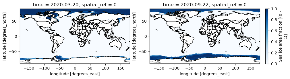
nDarray example 3: ERA5 atmospheric reanalysis

Read data

era5_ds = xarray.open_zarr(
    "gs://gcp-public-data-arco-era5/ar/1959-2022-full_37-1h-0p25deg-chunk-1.zarr-v2",
    chunks={'time': 48},
    consolidated=True,
    storage_options=dict(token='anon'),
    
)

def ds_swaplon(ds):
    return ds.assign_coords(longitude=(((ds.longitude + 180) % 360) - 180)).sortby('longitude')

era5_ds = ds_swaplon(era5_ds).rio.write_crs('EPSG:4326')

Preview data structure

era5_ds

<xarray.Dataset> Size: 534TB
Dimensions:                                           (time: 552264,
                                                       latitude: 721,
                                                       longitude: 1440,
                                                       level: 37)
Coordinates:
  * latitude                                          (latitude) float32 3kB ...
  * level                                             (level) int64 296B 1 .....
  * time                                              (time) datetime64[ns] 4MB ...
  * longitude                                         (longitude) float32 6kB ...
    spatial_ref                                       int64 8B 0
Data variables: (12/31)
    10m_u_component_of_wind                           (time, latitude, longitude) float32 2TB dask.array<chunksize=(48, 721, 1440), meta=np.ndarray>
    10m_v_component_of_wind                           (time, latitude, longitude) float32 2TB dask.array<chunksize=(48, 721, 1440), meta=np.ndarray>
    2m_temperature                                    (time, latitude, longitude) float32 2TB dask.array<chunksize=(48, 721, 1440), meta=np.ndarray>
    angle_of_sub_gridscale_orography                  (latitude, longitude) float32 4MB dask.array<chunksize=(721, 1440), meta=np.ndarray>
    anisotropy_of_sub_gridscale_orography             (latitude, longitude) float32 4MB dask.array<chunksize=(721, 1440), meta=np.ndarray>
    geopotential                                      (time, level, latitude, longitude) float32 85TB dask.array<chunksize=(48, 37, 721, 1440), meta=np.ndarray>
    ...                                                ...
    total_precipitation                               (time, latitude, longitude) float32 2TB dask.array<chunksize=(48, 721, 1440), meta=np.ndarray>
    type_of_high_vegetation                           (latitude, longitude) float32 4MB dask.array<chunksize=(721, 1440), meta=np.ndarray>
    type_of_low_vegetation                            (latitude, longitude) float32 4MB dask.array<chunksize=(721, 1440), meta=np.ndarray>
    u_component_of_wind                               (time, level, latitude, longitude) float32 85TB dask.array<chunksize=(48, 37, 721, 1440), meta=np.ndarray>
    v_component_of_wind                               (time, level, latitude, longitude) float32 85TB dask.array<chunksize=(48, 37, 721, 1440), meta=np.ndarray>
    vertical_velocity                                 (time, level, latitude, longitude) float32 85TB dask.array<chunksize=(48, 37, 721, 1440), meta=np.ndarray>

xarray.Dataset

• Dimensions:
  • time: 552264
  • latitude: 721
  • longitude: 1440
  • level: 37
• Coordinates: (5)
  • latitude
    (latitude)
    float32
    90.0 89.75 89.5 ... -89.75 -90.0

    long_name :

    latitude

    units :

    degrees_north

    array([ 90.  ,  89.75,  89.5 , ..., -89.5 , -89.75, -90.  ], dtype=float32)

  • level
    (level)
    int64
    1 2 3 5 7 ... 900 925 950 975 1000

    array([   1,    2,    3,    5,    7,   10,   20,   30,   50,   70,  100,  125,
            150,  175,  200,  225,  250,  300,  350,  400,  450,  500,  550,  600,
            650,  700,  750,  775,  800,  825,  850,  875,  900,  925,  950,  975,
           1000])

  • time
    (time)
    datetime64[ns]
    1959-01-01 ... 2021-12-31T23:00:00

    array(['1959-01-01T00:00:00.000000000', '1959-01-01T01:00:00.000000000',
           '1959-01-01T02:00:00.000000000', ..., '2021-12-31T21:00:00.000000000',
           '2021-12-31T22:00:00.000000000', '2021-12-31T23:00:00.000000000'],
          dtype='datetime64[ns]')

  • longitude
    (longitude)
    float32
    -180.0 -179.8 ... 179.5 179.8

    long_name :

    longitude

    units :

    degrees_east

    array([-180.  , -179.75, -179.5 , ...,  179.25,  179.5 ,  179.75],
          dtype=float32)

  • spatial_ref
    ()
    int64
    0

    crs_wkt :

    GEOGCS["WGS 84",DATUM["WGS_1984",SPHEROID["WGS 84",6378137,298.257223563,AUTHORITY["EPSG","7030"]],AUTHORITY["EPSG","6326"]],PRIMEM["Greenwich",0,AUTHORITY["EPSG","8901"]],UNIT["degree",0.0174532925199433,AUTHORITY["EPSG","9122"]],AXIS["Latitude",NORTH],AXIS["Longitude",EAST],AUTHORITY["EPSG","4326"]]

    semi_major_axis :

    6378137.0

    semi_minor_axis :

    6356752.314245179

    inverse_flattening :

    298.257223563

    reference_ellipsoid_name :

    WGS 84

    longitude_of_prime_meridian :

    0.0

    prime_meridian_name :

    Greenwich

    geographic_crs_name :

    WGS 84

    horizontal_datum_name :

    World Geodetic System 1984

    grid_mapping_name :

    latitude_longitude

    spatial_ref :

    GEOGCS["WGS 84",DATUM["WGS_1984",SPHEROID["WGS 84",6378137,298.257223563,AUTHORITY["EPSG","7030"]],AUTHORITY["EPSG","6326"]],PRIMEM["Greenwich",0,AUTHORITY["EPSG","8901"]],UNIT["degree",0.0174532925199433,AUTHORITY["EPSG","9122"]],AXIS["Latitude",NORTH],AXIS["Longitude",EAST],AUTHORITY["EPSG","4326"]]

    array(0)

• Data variables: (31)
  • 10m_u_component_of_wind
    (time, latitude, longitude)
    float32
    dask.array<chunksize=(48, 721, 1440), meta=np.ndarray>

    long_name :

    10 metre U wind component

    short_name :

    u10

    units :

    m s**-1

    Array Chunk Bytes 2.09 TiB 190.11 MiB Shape (552264, 721, 1440) (48, 721, 1440) Dask graph 11506 chunks in 3 graph layers Data type float32 numpy.ndarray

  • 10m_v_component_of_wind
    (time, latitude, longitude)
    float32
    dask.array<chunksize=(48, 721, 1440), meta=np.ndarray>

    long_name :

    10 metre V wind component

    short_name :

    v10

    units :

    m s**-1

    Array Chunk Bytes 2.09 TiB 190.11 MiB Shape (552264, 721, 1440) (48, 721, 1440) Dask graph 11506 chunks in 3 graph layers Data type float32 numpy.ndarray

  • 2m_temperature
    (time, latitude, longitude)
    float32
    dask.array<chunksize=(48, 721, 1440), meta=np.ndarray>

    long_name :

    2 metre temperature

    short_name :

    t2m

    units :

    K

    Array Chunk Bytes 2.09 TiB 190.11 MiB Shape (552264, 721, 1440) (48, 721, 1440) Dask graph 11506 chunks in 3 graph layers Data type float32 numpy.ndarray

  • angle_of_sub_gridscale_orography
    (latitude, longitude)
    float32
    dask.array<chunksize=(721, 1440), meta=np.ndarray>

    long_name :

    Angle of sub-gridscale orography

    short_name :

    anor

    units :

    radians

    Array Chunk Bytes 3.96 MiB 3.96 MiB Shape (721, 1440) (721, 1440) Dask graph 1 chunks in 3 graph layers Data type float32 numpy.ndarray

  • anisotropy_of_sub_gridscale_orography
    (latitude, longitude)
    float32
    dask.array<chunksize=(721, 1440), meta=np.ndarray>

    long_name :

    Anisotropy of sub-gridscale orography

    short_name :

    isor

    units :

    ~

    Array Chunk Bytes 3.96 MiB 3.96 MiB Shape (721, 1440) (721, 1440) Dask graph 1 chunks in 3 graph layers Data type float32 numpy.ndarray

  • geopotential
    (time, level, latitude, longitude)
    float32
    dask.array<chunksize=(48, 37, 721, 1440), meta=np.ndarray>

    long_name :

    Geopotential

    short_name :

    z

    standard_name :

    geopotential

    units :

    m**2 s**-2

    Array Chunk Bytes 77.18 TiB 6.87 GiB Shape (552264, 37, 721, 1440) (48, 37, 721, 1440) Dask graph 11506 chunks in 3 graph layers Data type float32 numpy.ndarray

  • geopotential_at_surface
    (latitude, longitude)
    float32
    dask.array<chunksize=(721, 1440), meta=np.ndarray>

    long_name :

    Geopotential

    short_name :

    z

    standard_name :

    geopotential

    units :

    m**2 s**-2

    Array Chunk Bytes 3.96 MiB 3.96 MiB Shape (721, 1440) (721, 1440) Dask graph 1 chunks in 3 graph layers Data type float32 numpy.ndarray

  • high_vegetation_cover
    (latitude, longitude)
    float32
    dask.array<chunksize=(721, 1440), meta=np.ndarray>

    long_name :

    High vegetation cover

    short_name :

    cvh

    units :

    (0 - 1)

    Array Chunk Bytes 3.96 MiB 3.96 MiB Shape (721, 1440) (721, 1440) Dask graph 1 chunks in 3 graph layers Data type float32 numpy.ndarray

  • lake_cover
    (latitude, longitude)
    float32
    dask.array<chunksize=(721, 1440), meta=np.ndarray>

    long_name :

    Lake cover

    short_name :

    cl

    units :

    (0 - 1)

    Array Chunk Bytes 3.96 MiB 3.96 MiB Shape (721, 1440) (721, 1440) Dask graph 1 chunks in 3 graph layers Data type float32 numpy.ndarray

  • lake_depth
    (latitude, longitude)
    float32
    dask.array<chunksize=(721, 1440), meta=np.ndarray>

    long_name :

    Lake total depth

    short_name :

    dl

    units :

    m

    Array Chunk Bytes 3.96 MiB 3.96 MiB Shape (721, 1440) (721, 1440) Dask graph 1 chunks in 3 graph layers Data type float32 numpy.ndarray

  • land_sea_mask
    (latitude, longitude)
    float32
    dask.array<chunksize=(721, 1440), meta=np.ndarray>

    long_name :

    Land-sea mask

    short_name :

    lsm

    standard_name :

    land_binary_mask

    units :

    (0 - 1)

    Array Chunk Bytes 3.96 MiB 3.96 MiB Shape (721, 1440) (721, 1440) Dask graph 1 chunks in 3 graph layers Data type float32 numpy.ndarray

  • low_vegetation_cover
    (latitude, longitude)
    float32
    dask.array<chunksize=(721, 1440), meta=np.ndarray>

    long_name :

    Low vegetation cover

    short_name :

    cvl

    units :

    (0 - 1)

    Array Chunk Bytes 3.96 MiB 3.96 MiB Shape (721, 1440) (721, 1440) Dask graph 1 chunks in 3 graph layers Data type float32 numpy.ndarray

  • mean_sea_level_pressure
    (time, latitude, longitude)
    float32
    dask.array<chunksize=(48, 721, 1440), meta=np.ndarray>

    long_name :

    Mean sea level pressure

    short_name :

    msl

    standard_name :

    air_pressure_at_mean_sea_level

    units :

    Pa

    Array Chunk Bytes 2.09 TiB 190.11 MiB Shape (552264, 721, 1440) (48, 721, 1440) Dask graph 11506 chunks in 3 graph layers Data type float32 numpy.ndarray

  • sea_ice_cover
    (time, latitude, longitude)
    float32
    dask.array<chunksize=(48, 721, 1440), meta=np.ndarray>

    long_name :

    Sea ice area fraction

    short_name :

    siconc

    standard_name :

    sea_ice_area_fraction

    units :

    (0 - 1)

    Array Chunk Bytes 2.09 TiB 190.11 MiB Shape (552264, 721, 1440) (48, 721, 1440) Dask graph 11506 chunks in 3 graph layers Data type float32 numpy.ndarray

  • sea_surface_temperature
    (time, latitude, longitude)
    float32
    dask.array<chunksize=(48, 721, 1440), meta=np.ndarray>

    long_name :

    Sea surface temperature

    short_name :

    sst

    units :

    K

    Array Chunk Bytes 2.09 TiB 190.11 MiB Shape (552264, 721, 1440) (48, 721, 1440) Dask graph 11506 chunks in 3 graph layers Data type float32 numpy.ndarray

  • slope_of_sub_gridscale_orography
    (latitude, longitude)
    float32
    dask.array<chunksize=(721, 1440), meta=np.ndarray>

    long_name :

    Slope of sub-gridscale orography

    short_name :

    slor

    units :

    ~

    Array Chunk Bytes 3.96 MiB 3.96 MiB Shape (721, 1440) (721, 1440) Dask graph 1 chunks in 3 graph layers Data type float32 numpy.ndarray

  • soil_type
    (latitude, longitude)
    float32
    dask.array<chunksize=(721, 1440), meta=np.ndarray>

    long_name :

    Soil type

    short_name :

    slt

    units :

    ~

    Array Chunk Bytes 3.96 MiB 3.96 MiB Shape (721, 1440) (721, 1440) Dask graph 1 chunks in 3 graph layers Data type float32 numpy.ndarray

  • specific_humidity
    (time, level, latitude, longitude)
    float32
    dask.array<chunksize=(48, 37, 721, 1440), meta=np.ndarray>

    long_name :

    Specific humidity

    short_name :

    q

    standard_name :

    specific_humidity

    units :

    kg kg**-1

    Array Chunk Bytes 77.18 TiB 6.87 GiB Shape (552264, 37, 721, 1440) (48, 37, 721, 1440) Dask graph 11506 chunks in 3 graph layers Data type float32 numpy.ndarray

  • standard_deviation_of_filtered_subgrid_orography
    (latitude, longitude)
    float32
    dask.array<chunksize=(721, 1440), meta=np.ndarray>

    long_name :

    Standard deviation of filtered subgrid orography

    short_name :

    sdfor

    units :

    m

    Array Chunk Bytes 3.96 MiB 3.96 MiB Shape (721, 1440) (721, 1440) Dask graph 1 chunks in 3 graph layers Data type float32 numpy.ndarray

  • standard_deviation_of_orography
    (latitude, longitude)
    float32
    dask.array<chunksize=(721, 1440), meta=np.ndarray>

    long_name :

    Standard deviation of orography

    short_name :

    sdor

    units :

    m

    Array Chunk Bytes 3.96 MiB 3.96 MiB Shape (721, 1440) (721, 1440) Dask graph 1 chunks in 3 graph layers Data type float32 numpy.ndarray

  • surface_pressure
    (time, latitude, longitude)
    float32
    dask.array<chunksize=(48, 721, 1440), meta=np.ndarray>

    long_name :

    Surface pressure

    short_name :

    sp

    standard_name :

    surface_air_pressure

    units :

    Pa

    Array Chunk Bytes 2.09 TiB 190.11 MiB Shape (552264, 721, 1440) (48, 721, 1440) Dask graph 11506 chunks in 3 graph layers Data type float32 numpy.ndarray

  • temperature
    (time, level, latitude, longitude)
    float32
    dask.array<chunksize=(48, 37, 721, 1440), meta=np.ndarray>

    long_name :

    Temperature

    short_name :

    t

    standard_name :

    air_temperature

    units :

    K

    Array Chunk Bytes 77.18 TiB 6.87 GiB Shape (552264, 37, 721, 1440) (48, 37, 721, 1440) Dask graph 11506 chunks in 3 graph layers Data type float32 numpy.ndarray

  • toa_incident_solar_radiation
    (time, latitude, longitude)
    float32
    dask.array<chunksize=(48, 721, 1440), meta=np.ndarray>

    long_name :

    TOA incident solar radiation

    short_name :

    tisr

    units :

    J m**-2

    Array Chunk Bytes 2.09 TiB 190.11 MiB Shape (552264, 721, 1440) (48, 721, 1440) Dask graph 11506 chunks in 3 graph layers Data type float32 numpy.ndarray

  • total_cloud_cover
    (time, latitude, longitude)
    float32
    dask.array<chunksize=(48, 721, 1440), meta=np.ndarray>

    long_name :

    Total cloud cover

    short_name :

    tcc

    standard_name :

    cloud_area_fraction

    units :

    (0 - 1)

    Array Chunk Bytes 2.09 TiB 190.11 MiB Shape (552264, 721, 1440) (48, 721, 1440) Dask graph 11506 chunks in 3 graph layers Data type float32 numpy.ndarray

  • total_column_water_vapour
    (time, latitude, longitude)
    float32
    dask.array<chunksize=(48, 721, 1440), meta=np.ndarray>

    long_name :

    Total column vertically-integrated water vapour

    short_name :

    tcwv

    standard_name :

    lwe_thickness_of_atmosphere_mass_content_of_water_vapor

    units :

    kg m**-2

    Array Chunk Bytes 2.09 TiB 190.11 MiB Shape (552264, 721, 1440) (48, 721, 1440) Dask graph 11506 chunks in 3 graph layers Data type float32 numpy.ndarray

  • total_precipitation
    (time, latitude, longitude)
    float32
    dask.array<chunksize=(48, 721, 1440), meta=np.ndarray>

    long_name :

    Total precipitation

    short_name :

    tp

    units :

    m

    Array Chunk Bytes 2.09 TiB 190.11 MiB Shape (552264, 721, 1440) (48, 721, 1440) Dask graph 11506 chunks in 3 graph layers Data type float32 numpy.ndarray

  • type_of_high_vegetation
    (latitude, longitude)
    float32
    dask.array<chunksize=(721, 1440), meta=np.ndarray>

    long_name :

    Type of high vegetation

    short_name :

    tvh

    units :

    ~

    Array Chunk Bytes 3.96 MiB 3.96 MiB Shape (721, 1440) (721, 1440) Dask graph 1 chunks in 3 graph layers Data type float32 numpy.ndarray

  • type_of_low_vegetation
    (latitude, longitude)
    float32
    dask.array<chunksize=(721, 1440), meta=np.ndarray>

    long_name :

    Type of low vegetation

    short_name :

    tvl

    units :

    ~

    Array Chunk Bytes 3.96 MiB 3.96 MiB Shape (721, 1440) (721, 1440) Dask graph 1 chunks in 3 graph layers Data type float32 numpy.ndarray

  • u_component_of_wind
    (time, level, latitude, longitude)
    float32
    dask.array<chunksize=(48, 37, 721, 1440), meta=np.ndarray>

    long_name :

    U component of wind

    short_name :

    u

    standard_name :

    eastward_wind

    units :

    m s**-1

    Array Chunk Bytes 77.18 TiB 6.87 GiB Shape (552264, 37, 721, 1440) (48, 37, 721, 1440) Dask graph 11506 chunks in 3 graph layers Data type float32 numpy.ndarray

  • v_component_of_wind
    (time, level, latitude, longitude)
    float32
    dask.array<chunksize=(48, 37, 721, 1440), meta=np.ndarray>

    long_name :

    V component of wind

    short_name :

    v

    standard_name :

    northward_wind

    units :

    m s**-1

    Array Chunk Bytes 77.18 TiB 6.87 GiB Shape (552264, 37, 721, 1440) (48, 37, 721, 1440) Dask graph 11506 chunks in 3 graph layers Data type float32 numpy.ndarray

  • vertical_velocity
    (time, level, latitude, longitude)
    float32
    dask.array<chunksize=(48, 37, 721, 1440), meta=np.ndarray>

    long_name :

    Vertical velocity

    short_name :

    w

    standard_name :

    lagrangian_tendency_of_air_pressure

    units :

    Pa s**-1

    Array Chunk Bytes 77.18 TiB 6.87 GiB Shape (552264, 37, 721, 1440) (48, 37, 721, 1440) Dask graph 11506 chunks in 3 graph layers Data type float32 numpy.ndarray

• Indexes: (4)
  • latitude
    PandasIndex

    PandasIndex(Index([  90.0,  89.75,   89.5,  89.25,   89.0,  88.75,   88.5,  88.25,   88.0,
            87.75,
           ...
           -87.75,  -88.0, -88.25,  -88.5, -88.75,  -89.0, -89.25,  -89.5, -89.75,
            -90.0],
          dtype='float32', name='latitude', length=721))

  • level
    PandasIndex

    PandasIndex(Index([   1,    2,    3,    5,    7,   10,   20,   30,   50,   70,  100,  125,
            150,  175,  200,  225,  250,  300,  350,  400,  450,  500,  550,  600,
            650,  700,  750,  775,  800,  825,  850,  875,  900,  925,  950,  975,
           1000],
          dtype='int64', name='level'))

  • time
    PandasIndex

    PandasIndex(DatetimeIndex(['1959-01-01 00:00:00', '1959-01-01 01:00:00',
                   '1959-01-01 02:00:00', '1959-01-01 03:00:00',
                   '1959-01-01 04:00:00', '1959-01-01 05:00:00',
                   '1959-01-01 06:00:00', '1959-01-01 07:00:00',
                   '1959-01-01 08:00:00', '1959-01-01 09:00:00',
                   ...
                   '2021-12-31 14:00:00', '2021-12-31 15:00:00',
                   '2021-12-31 16:00:00', '2021-12-31 17:00:00',
                   '2021-12-31 18:00:00', '2021-12-31 19:00:00',
                   '2021-12-31 20:00:00', '2021-12-31 21:00:00',
                   '2021-12-31 22:00:00', '2021-12-31 23:00:00'],
                  dtype='datetime64[ns]', name='time', length=552264, freq=None))

  • longitude
    PandasIndex

    PandasIndex(Index([ -180.0, -179.75,  -179.5, -179.25,  -179.0, -178.75,  -178.5, -178.25,
            -178.0, -177.75,
           ...
             177.5,  177.75,   178.0,  178.25,   178.5,  178.75,   179.0,  179.25,
             179.5,  179.75],
          dtype='float32', name='longitude', length=1440))

• Attributes: (0)

Visualize data

f,axs=plt.subplots(1,2,figsize=(10,7),layout='compressed')
era5_ds['sea_ice_cover'].sel(time='2020-03-20T00').plot(ax=axs[0],cmap='Blues',add_colorbar=False)
era5_ds['sea_ice_cover'].sel(time='2020-09-22T00').plot(ax=axs[1],cmap='Blues')

for ax in axs:
    world_gdf.boundary.plot(ax=ax,linewidth=1,color='black')

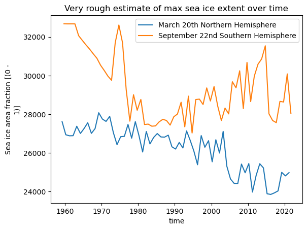
march20_seaice_extent_da = era5_ds['sea_ice_cover'].sel(time=((era5_ds.time.dt.month == 3) & 
          (era5_ds.time.dt.day == 20) & 
          (era5_ds.time.dt.hour == 1))
).rio.reproject('EPSG:6933')

sept22_seaice_extent_da = era5_ds['sea_ice_cover'].sel(time=((era5_ds.time.dt.month == 9) & 
          (era5_ds.time.dt.day == 22) & 
          (era5_ds.time.dt.hour == 1))
).rio.reproject('EPSG:6933')

march20_max_seaice_extent_NH_da = march20_seaice_extent_da.where(march20_seaice_extent_da.y>0).sum(dim=['x','y']).compute()
sept22_max_seaice_extent_SH_da = sept22_seaice_extent_da.where(sept22_seaice_extent_da.y<0).sum(dim=['x','y']).compute()

f,ax=plt.subplots()
march20_max_seaice_extent_NH_da.plot(ax=ax,label='March 20th Northern Hemisphere')
sept22_max_seaice_extent_SH_da.plot(ax=ax, label='September 22nd Southern Hemisphere')
ax.legend()
ax.set_title('Very rough estimate of max sea ice extent over time')

Text(0.5, 1.0, 'Very rough estimate of max sea ice extent over time')

That’s all, thanks for checking out this notebook!