07 PCA/EOF analysis demo#
UW Geospatial Data Analysis
CEE467/CEWA567
David Shean, Eric Gagliano, Quinn Brencher
Overview#
PCA/EOF analysis is great way to analyze variability in time series data. We will be using EOFs on the ERA5 anomaly data from this weeks lab in order to analyze climate modes. Here is an explainer on EOF analyis as it relates to climate data. We will be using xeofs, a package for xarray PCA analysis Check out the xeofs example gallery for the different types of analysis.
Additional examples of PCA/SVD/EOFs with different packages
For more comprehensive details on EOF analysis as it relates to climate data, check out A Primer for EOF Analysis of Climate Data.
#!pip install xeofs
from pathlib import Path
import xarray as xr
import geopandas as gpd
import matplotlib.pyplot as plt
from matplotlib.gridspec import GridSpec
import cartopy.crs as ccrs
import os
import xeofs
Read in data, coarsen, and reproject#
era5_data_dir = f'{Path.home()}/gda_demo_data/era5_data'
anom_fn = os.path.join(era5_data_dir, '1month_anomaly_Global_ea_2t.nc')
anom_ds = xr.open_dataset(anom_fn, chunks='auto')
# anom_ds = anom_ds.resample(time='YE').mean()
# anom_ds
def ds_swaplon(ds):
    return ds.assign_coords(longitude=(((ds.longitude + 180) % 360) - 180)).sortby('longitude')

anom_ds = ds_swaplon(anom_ds)

anom_ds.rio.write_crs('EPSG:4326', inplace=True);
anom_ds
<xarray.Dataset> Size: 2GB
Dimensions:      (time: 517, latitude: 721, longitude: 1440)
Coordinates:
  * time         (time) datetime64[ns] 4kB 1979-01-01 1979-02-01 ... 2022-01-01
  * latitude     (latitude) float64 6kB 90.0 89.75 89.5 ... -89.5 -89.75 -90.0
  * longitude    (longitude) float64 12kB -180.0 -179.8 -179.5 ... 179.5 179.8
    spatial_ref  int64 8B 0
Data variables:
    t2m          (time, latitude, longitude) float32 2GB dask.array<chunksize=(205, 286, 480), meta=np.ndarray>
Attributes:
    GRIB_edition:            1
    GRIB_centre:             ecmf
    GRIB_centreDescription:  European Centre for Medium-Range Weather Forecasts
    GRIB_subCentre:          0
    Conventions:             CF-1.7
    institution:             European Centre for Medium-Range Weather Forecasts
history: 2022-02-28T07:59 GRIB to CDM+CF via cfgrib-0.9.1...anom_ds = anom_ds.coarsen(latitude=2, longitude=4, boundary='trim').mean()
anom_ds
<xarray.Dataset> Size: 268MB
Dimensions:      (time: 517, latitude: 360, longitude: 360)
Coordinates:
  * time         (time) datetime64[ns] 4kB 1979-01-01 1979-02-01 ... 2022-01-01
  * latitude     (latitude) float64 3kB 89.88 89.38 88.88 ... -89.12 -89.62
  * longitude    (longitude) float64 3kB -179.6 -178.6 -177.6 ... 178.4 179.4
    spatial_ref  int64 8B 0
Data variables:
    t2m          (time, latitude, longitude) float32 268MB dask.array<chunksize=(205, 143, 120), meta=np.ndarray>
Attributes:
    GRIB_edition:            1
    GRIB_centre:             ecmf
    GRIB_centreDescription:  European Centre for Medium-Range Weather Forecasts
    GRIB_subCentre:          0
    Conventions:             CF-1.7
    institution:             European Centre for Medium-Range Weather Forecasts
history: 2022-02-28T07:59 GRIB to CDM+CF via cfgrib-0.9.1...ea_proj = '+proj=moll'
anom_da = anom_ds['t2m'].rio.reproject(ea_proj)
anom_da
<xarray.DataArray 't2m' (time: 517, y: 228, x: 455)> Size: 215MB
array([[[nan, nan, nan, ..., nan, nan, nan],
        [nan, nan, nan, ..., nan, nan, nan],
        [nan, nan, nan, ..., nan, nan, nan],
        ...,
        [nan, nan, nan, ..., nan, nan, nan],
        [nan, nan, nan, ..., nan, nan, nan],
        [nan, nan, nan, ..., nan, nan, nan]],

       [[nan, nan, nan, ..., nan, nan, nan],
        [nan, nan, nan, ..., nan, nan, nan],
        [nan, nan, nan, ..., nan, nan, nan],
        ...,
        [nan, nan, nan, ..., nan, nan, nan],
        [nan, nan, nan, ..., nan, nan, nan],
        [nan, nan, nan, ..., nan, nan, nan]],

       [[nan, nan, nan, ..., nan, nan, nan],
        [nan, nan, nan, ..., nan, nan, nan],
        [nan, nan, nan, ..., nan, nan, nan],
        ...,
...
        ...,
        [nan, nan, nan, ..., nan, nan, nan],
        [nan, nan, nan, ..., nan, nan, nan],
        [nan, nan, nan, ..., nan, nan, nan]],

       [[nan, nan, nan, ..., nan, nan, nan],
        [nan, nan, nan, ..., nan, nan, nan],
        [nan, nan, nan, ..., nan, nan, nan],
        ...,
        [nan, nan, nan, ..., nan, nan, nan],
        [nan, nan, nan, ..., nan, nan, nan],
        [nan, nan, nan, ..., nan, nan, nan]],

       [[nan, nan, nan, ..., nan, nan, nan],
        [nan, nan, nan, ..., nan, nan, nan],
        [nan, nan, nan, ..., nan, nan, nan],
        ...,
        [nan, nan, nan, ..., nan, nan, nan],
        [nan, nan, nan, ..., nan, nan, nan],
        [nan, nan, nan, ..., nan, nan, nan]]], dtype=float32)
Coordinates:
  * x            (x) float64 4kB -1.8e+07 -1.792e+07 ... 1.789e+07 1.797e+07
  * y            (y) float64 2kB 8.981e+06 8.902e+06 ... -8.847e+06 -8.926e+06
  * time         (time) datetime64[ns] 4kB 1979-01-01 1979-02-01 ... 2022-01-01
    spatial_ref  int64 8B 0
Attributes: (12/30)
    GRIB_paramId:                             167
    GRIB_dataType:                            an
    GRIB_numberOfPoints:                      1038240
    GRIB_typeOfLevel:                         surface
    GRIB_stepUnits:                           1
    GRIB_stepType:                            avgua
    ...                                       ...
    GRIB_shortName:                           2t
    GRIB_totalNumber:                         0
    GRIB_units:                               K
    long_name:                                2 metre temperature
    units:                                    K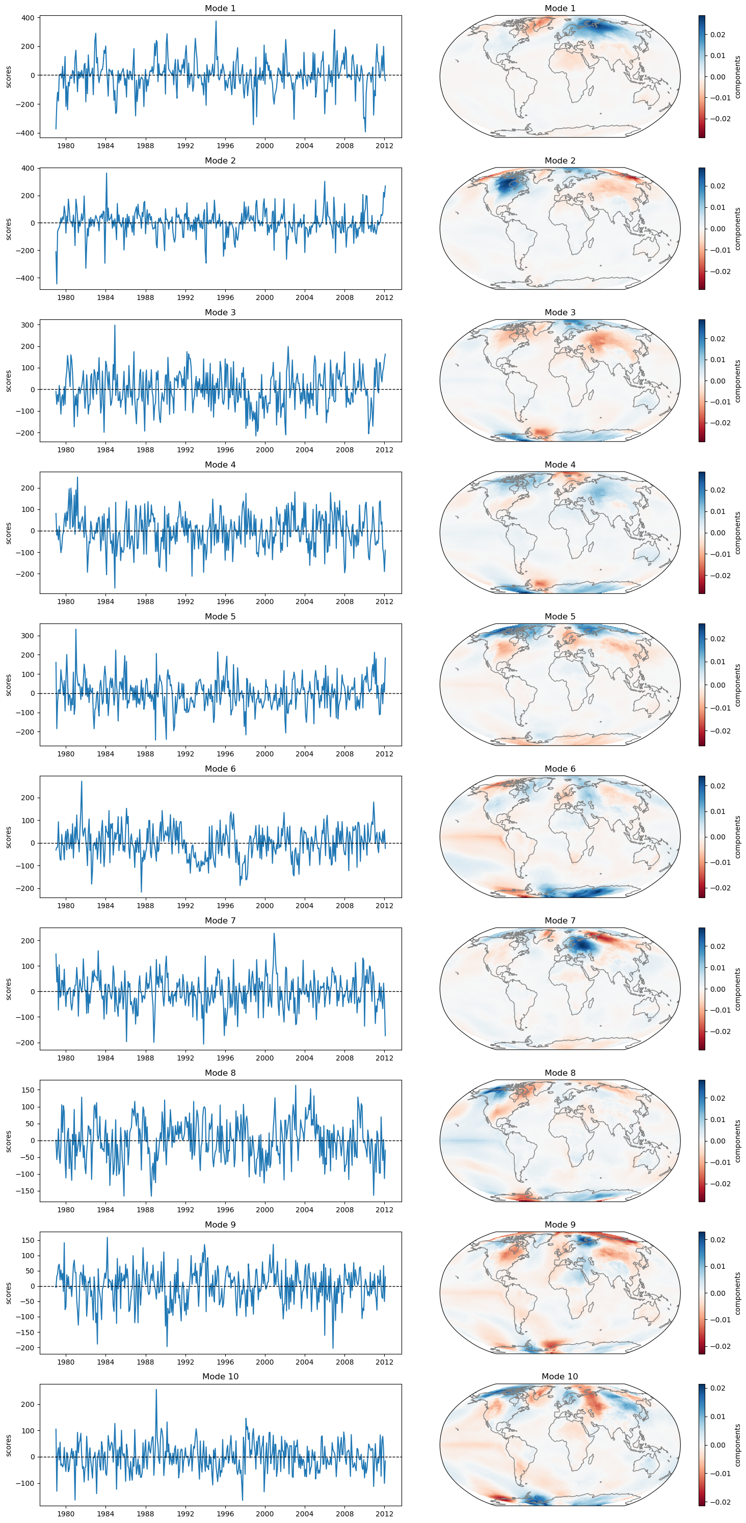
standard_name: unknownNow try performing the EOF analysis…#
eof = xeofs.single.EOF(n_modes=10)
eof.fit(anom_da, dim="time")
eof.explained_variance_ratio()
components = eof.components()
scores = eof.scores()
n = len(scores.mode)

kwargs = {"cmap": "RdBu"}#, "vmin": -0.05, "vmax": 0.05}

f = plt.figure(figsize=(15, 3*n))
gs = GridSpec(n, 2, width_ratios=[2, 2])
ax0 = [f.add_subplot(gs[i, 0]) for i in range(n)]
ax1 = [f.add_subplot(gs[i, 1], projection=ccrs.Robinson()) for i in range(n)]

for i, (a0, a1) in enumerate(zip(ax0, ax1)):
    scores.sel(mode=i + 1).plot(ax=a0)
    a0.axhline(0, color="k", linestyle='--', lw=1)
    a1.coastlines(color=".5")
    components.sel(mode=i + 1).plot(ax=a1, **kwargs)

    a0.set_xlabel("")

f.tight_layout()
Whooops, looks like the leading pattern is dominated by the global warming signal! Let’s subtract out this trend with extended EOF analysis…#
# Could also try to remove the linear trend from the data before running the EOF analysis, though this assumes the trend is linear
# polyfit_coeffs_da = anom_da.polyfit(deg=1,dim='time')['polyfit_coefficients']
# anom_polyfit_da = xr.polyval(anom_da.time, polyfit_coeffs_da)
# anom_da = anom_da - anom_polyfit_da
# anom_da

# eof = xeofs.single.EOF(n_modes=10)
# eof.fit(anom_da, dim="time")
# eof.explained_variance_ratio()
# components = eof.components()
# scores = eof.scores()
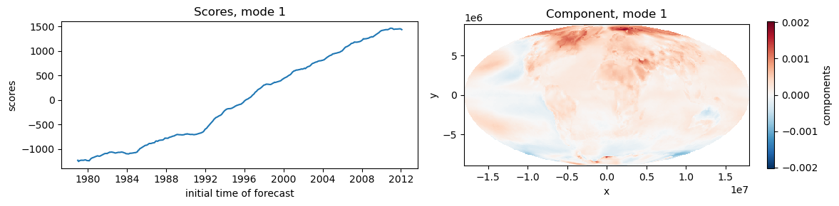
eeof = xeofs.single.ExtendedEOF(n_modes=5, tau=1, embedding=120, n_pca_modes=50)
eeof.fit(anom_da, dim="time")
components_ext = eeof.components()
scores_ext = eeof.scores()
f, axs = plt.subplots(1, 2, figsize=(12, 3))
scores_ext.sel(mode=1).plot(ax=axs[0])
components_ext.sel(mode=1, embedding=0).plot(ax=axs[1])
axs[1].set_aspect('equal')

axs[0].set_title("Scores, mode 1")
axs[1].set_title("Component, mode 1")

f.tight_layout()
anom_trends_da = eeof.inverse_transform(scores_ext.sel(mode=1))
anom_detrended_da = anom_da - anom_trends_da
anom_detrended_da
<xarray.DataArray (time: 517, y: 228, x: 455)> Size: 429MB
array([[[nan, nan, nan, ..., nan, nan, nan],
        [nan, nan, nan, ..., nan, nan, nan],
        [nan, nan, nan, ..., nan, nan, nan],
        ...,
        [nan, nan, nan, ..., nan, nan, nan],
        [nan, nan, nan, ..., nan, nan, nan],
        [nan, nan, nan, ..., nan, nan, nan]],

       [[nan, nan, nan, ..., nan, nan, nan],
        [nan, nan, nan, ..., nan, nan, nan],
        [nan, nan, nan, ..., nan, nan, nan],
        ...,
        [nan, nan, nan, ..., nan, nan, nan],
        [nan, nan, nan, ..., nan, nan, nan],
        [nan, nan, nan, ..., nan, nan, nan]],

       [[nan, nan, nan, ..., nan, nan, nan],
        [nan, nan, nan, ..., nan, nan, nan],
        [nan, nan, nan, ..., nan, nan, nan],
        ...,
...
        ...,
        [nan, nan, nan, ..., nan, nan, nan],
        [nan, nan, nan, ..., nan, nan, nan],
        [nan, nan, nan, ..., nan, nan, nan]],

       [[nan, nan, nan, ..., nan, nan, nan],
        [nan, nan, nan, ..., nan, nan, nan],
        [nan, nan, nan, ..., nan, nan, nan],
        ...,
        [nan, nan, nan, ..., nan, nan, nan],
        [nan, nan, nan, ..., nan, nan, nan],
        [nan, nan, nan, ..., nan, nan, nan]],

       [[nan, nan, nan, ..., nan, nan, nan],
        [nan, nan, nan, ..., nan, nan, nan],
        [nan, nan, nan, ..., nan, nan, nan],
        ...,
        [nan, nan, nan, ..., nan, nan, nan],
        [nan, nan, nan, ..., nan, nan, nan],
        [nan, nan, nan, ..., nan, nan, nan]]])
Coordinates:
  * x            (x) float64 4kB -1.8e+07 -1.792e+07 ... 1.789e+07 1.797e+07
  * y            (y) float64 2kB 8.981e+06 8.902e+06 ... -8.847e+06 -8.926e+06
  * time         (time) datetime64[ns] 4kB 1979-01-01 1979-02-01 ... 2022-01-01
    spatial_ref  int64 8B 0
Attributes: (12/30)
    GRIB_paramId:                             167
    GRIB_dataType:                            an
    GRIB_numberOfPoints:                      1038240
    GRIB_typeOfLevel:                         surface
    GRIB_stepUnits:                           1
    GRIB_stepType:                            avgua
    ...                                       ...
    GRIB_shortName:                           2t
    GRIB_totalNumber:                         0
    GRIB_units:                               K
    long_name:                                2 metre temperature
    units:                                    K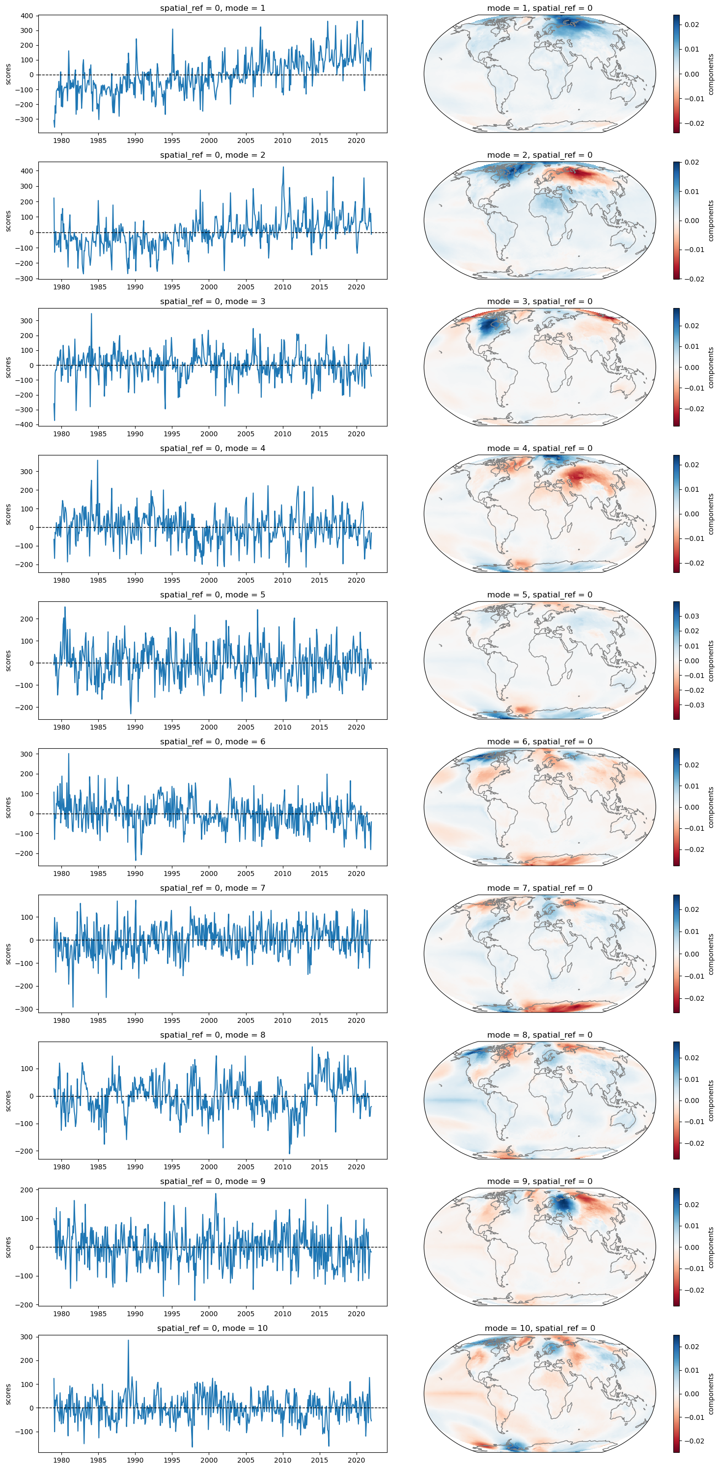
standard_name: unknownNow we can run the EOF analysis again on the detrended data…#
eof_model_detrended = xeofs.single.EOF(n_modes=10)
eof_model_detrended.fit(anom_detrended_da, dim="time")
scores_detrended = eof_model_detrended.scores()
components_detrended = eof_model_detrended.components()
n = len(scores_detrended.mode)

kwargs = {"cmap": "RdBu"}#, "vmin": -0.05, "vmax": 0.05}

f = plt.figure(figsize=(15, 3*n))
gs = GridSpec(n, 2, width_ratios=[2, 2])
ax0 = [f.add_subplot(gs[i, 0]) for i in range(n)]
ax1 = [f.add_subplot(gs[i, 1], projection=ccrs.Robinson()) for i in range(n)]

for i, (a0, a1) in enumerate(zip(ax0, ax1)):
    scores_detrended.sel(mode=i + 1).plot(ax=a0)
    a0.axhline(0, color="k", linestyle='--', lw=1)
    a1.coastlines(color=".5")
    components_detrended.sel(mode=i + 1).plot(ax=a1, **kwargs)

    a0.set_title(f"Mode {i + 1}")
    a1.set_title(f"Mode {i + 1}")
    a0.set_xlabel("")

f.tight_layout()