Lab 07 assignment (20 pts)#
UW Geospatial Data Analysis
CEE467/CEWA567
David Shean, Eric Gagliano, Quinn Brencher
Introduction#
Objectives#
Introduce xarray data model for N-d array analysis
Practice basic N-d array slicing, grouping and aggregation
Explore global and local climate reanalysis data
Instructions#
For each question or task below, write some code in the empty cell and execute to preserve your output
If you are in the graduate section of the class, please complete the challenge questions
Work together, consult resources we’ve discussed, post on slack!
Part 0: Imports and filenames#
First, let’s import the libraries we’ll need. Make sure to shut down any other kernels you have running!#
import os
from glob import glob
import numpy as np
import xarray as xr
import pandas as pd
import geopandas as gpd
import cartopy.crs as ccrs
import matplotlib.pyplot as plt
import holoviews as hv
import hvplot.xarray
import rioxarray
from pathlib import Path
import ee
import pyproj
era5_data_dir = f'{Path.home()}/gda_demo_data/era5_data'
# If you see no output for this cell, run the Jupyterbook demo notebook to query download data
!ls -lh $era5_data_dir
total 2.1G
-rw-r--r-- 1 eric eric 2.0G Feb 18 19:00 1month_anomaly_Global_ea_2t.nc
-rw-r--r-- 1 eric eric  48M Feb 18 18:58 climatology_0.25g_ea_2t.nc
Part 1: Global climatology (7 pts)#
Monthly temperature from 1979-2021#
Two datasets are provided:
Climatology - long-term mean monthly values from 1979-2021 (12 grids)
Anomaly - monthly difference from long-term monthly mean (505 grids from 1979-2021)
See here for more details on the datasets
Check out the download notebook for more information on how we prepared this data for you
Open the processed global monthly temperature anomaly and climatology NetCDF files#
clim_fn = os.path.join(era5_data_dir, 'climatology_0.25g_ea_2t.nc')
clim_ds = xr.open_dataset(clim_fn)
anom_fn = os.path.join(era5_data_dir, '1month_anomaly_Global_ea_2t.nc')
anom_ds = xr.open_dataset(anom_fn, chunks='auto')
Inspect the xarray Datasets#
Discuss with your neighbor
Review the output when you just type the DataSet name (similar to output from the
info()method)Note the number of time entries in each DataSet
What are the min and max longitude, min and max latitude
Note: The timestamp listed in the climatology dataset for each month is arbitrarily listed as 1981 (e.g., ‘1981-01-01’)
Remember these are mean values for each month of the year (12 total) across the entire 1979-2021 period
print info for the ‘t2m’ DataArray (temperature 2 m above ground)
clim_ds
<xarray.Dataset> Size: 50MB
Dimensions:    (time: 12, latitude: 721, longitude: 1440)
Coordinates:
  * time       (time) datetime64[ns] 96B 1981-01-01 1981-02-01 ... 1981-12-01
  * latitude   (latitude) float64 6kB 90.0 89.75 89.5 ... -89.5 -89.75 -90.0
  * longitude  (longitude) float64 12kB 0.0 0.25 0.5 0.75 ... 359.2 359.5 359.8
Data variables:
    t2m        (time, latitude, longitude) float32 50MB ...
Attributes:
    GRIB_edition:            1
    GRIB_centre:             ecmf
    GRIB_centreDescription:  European Centre for Medium-Range Weather Forecasts
    GRIB_subCentre:          0
    Conventions:             CF-1.7
    institution:             European Centre for Medium-Range Weather Forecasts
history: 2022-02-28T07:58 GRIB to CDM+CF via cfgrib-0.9.1...anom_ds
<xarray.Dataset> Size: 2GB
Dimensions: (time: 517, latitude: 721, longitude: 1440)
Coordinates:
* time (time) datetime64[ns] 4kB 1979-01-01 1979-02-01 ... 2022-01-01
* latitude (latitude) float64 6kB 90.0 89.75 89.5 ... -89.5 -89.75 -90.0
* longitude (longitude) float64 12kB 0.0 0.25 0.5 0.75 ... 359.2 359.5 359.8
Data variables:
t2m (time, latitude, longitude) float32 2GB dask.array<chunksize=(205, 286, 571), meta=np.ndarray>
Attributes:
GRIB_edition: 1
GRIB_centre: ecmf
GRIB_centreDescription: European Centre for Medium-Range Weather Forecasts
GRIB_subCentre: 0
Conventions: CF-1.7
institution: European Centre for Medium-Range Weather Forecasts
history: 2022-02-28T07:59 GRIB to CDM+CF via cfgrib-0.9.1...Written response: In your own words, briefly describe each dataset and what it might be used for. What are the data variables, and what is their data type? Please also note the spacing, min, and max of each coordinate for each dataset. What do you think chunks='auto' did in the open dataset call, and what might be its implications?#
STUDENT WRITTEN RESPONSE HERE
Convert the temperature values from K to C for the climatology dataset#
Note: don’t need to do this for anomalies, as they are relative values, not absolute
These operations are done on the DataArray level (not the top-level Dataset object level), so you’ll need to modify
clim_ds['t2m']Make sure you also update the units metadata attribute
The units used by xarray are stored in the clim_ds[‘t2m’].attrs dictionary
There is also a GRIB units variable, but this is holdover from the grib to xarray conversion–update it anyway!
Check
.attrsto make sure the attributes have been updatedCaution: Using
clim_ds['t2m'] = clim_ds['t2m'] - 273.15will remove the attributes, useclim_ds['t2m'] -= 273.15which does an in-place operation instead
# STUDENT CODE HERE
# STUDENT CODE HERE
{'GRIB_paramId': np.int64(167),
'GRIB_dataType': 'an',
'GRIB_numberOfPoints': np.int64(1038240),
'GRIB_typeOfLevel': 'surface',
'GRIB_stepUnits': np.int64(1),
'GRIB_stepType': 'avgua',
'GRIB_gridType': 'regular_ll',
'GRIB_NV': np.int64(0),
'GRIB_Nx': np.int64(1440),
'GRIB_Ny': np.int64(721),
'GRIB_cfName': 'unknown',
'GRIB_cfVarName': 't2m',
'GRIB_gridDefinitionDescription': 'Latitude/Longitude Grid',
'GRIB_iDirectionIncrementInDegrees': np.float64(0.25),
'GRIB_iScansNegatively': np.int64(0),
'GRIB_jDirectionIncrementInDegrees': np.float64(0.25),
'GRIB_jPointsAreConsecutive': np.int64(0),
'GRIB_jScansPositively': np.int64(0),
'GRIB_latitudeOfFirstGridPointInDegrees': np.float64(90.0),
'GRIB_latitudeOfLastGridPointInDegrees': np.float64(-90.0),
'GRIB_longitudeOfFirstGridPointInDegrees': np.float64(0.0),
'GRIB_longitudeOfLastGridPointInDegrees': np.float64(359.75),
'GRIB_missingValue': np.int64(9999),
'GRIB_name': '2 metre temperature',
'GRIB_shortName': '2t',
'GRIB_totalNumber': np.int64(0),
'GRIB_units': 'C',
'long_name': '2 metre temperature',
'units': 'C',
'standard_name': 'unknown'}
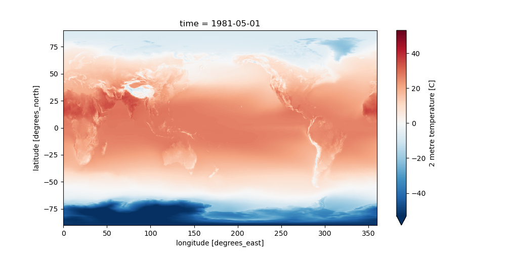
Check that these values seem reasonable with a quick plot of the May slice using isel()#
Review different strategies for selection here: http://xarray.pydata.org/en/stable/indexing.html
Try the
iselmethod with dimension name and integer index (e.g.,time=7)In the next step, you can use the
selmethod with dimension name and label (e.g.,time='2016-08-01', though the year may be different in your dataset)Note: the xarray convenience
plot.imshow()is much more efficient for regular grids than the defaultplot(), which usescontourfto interpolate values not on a regular gridSee the note here: https://xarray-test.readthedocs.io/en/latest/plotting.html#two-dimensions
Try the
robust=Trueoption
# STUDENT CODE HERE
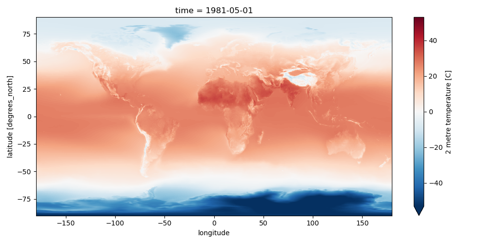
Set the longitude values to be (-180 to 180) instead of (0 to 360)#
Could also store as new set of coordinates called
longitude_180or something
def ds_swaplon(ds):
return ds.assign_coords(longitude=(((ds.longitude + 180) % 360) - 180)).sortby('longitude')
clim_ds = ds_swaplon(clim_ds)
anom_ds = ds_swaplon(anom_ds)
clim_ds.longitude
<xarray.DataArray 'longitude' (longitude: 1440)> Size: 12kB array([-180. , -179.75, -179.5 , ..., 179.25, 179.5 , 179.75]) Coordinates: * longitude (longitude) float64 12kB -180.0 -179.8 -179.5 ... 179.5 179.8
Now replot the May slice using .sel()#
#See time dimension index
clim_ds.time
<xarray.DataArray 'time' (time: 12)> Size: 96B
array(['1981-01-01T00:00:00.000000000', '1981-02-01T00:00:00.000000000',
       '1981-03-01T00:00:00.000000000', '1981-04-01T00:00:00.000000000',
       '1981-05-01T00:00:00.000000000', '1981-06-01T00:00:00.000000000',
       '1981-07-01T00:00:00.000000000', '1981-08-01T00:00:00.000000000',
       '1981-09-01T00:00:00.000000000', '1981-10-01T00:00:00.000000000',
       '1981-11-01T00:00:00.000000000', '1981-12-01T00:00:00.000000000'],
      dtype='datetime64[ns]')
Coordinates:
* time (time) datetime64[ns] 96B 1981-01-01 1981-02-01 ... 1981-12-01
Attributes:
long_name: initial time of forecast
standard_name: forecast_reference_time# STUDENT CODE HERE
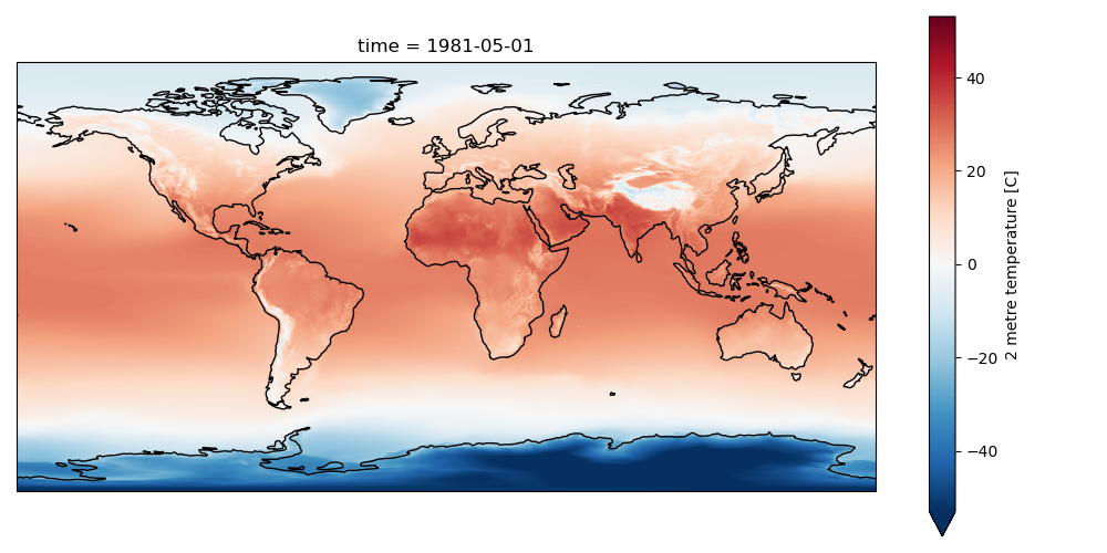
Create a plot for May, overlaying coastlines with cartopy#
Use a simple PlateCaree() projection as in example here:
https://scitools.org.uk/cartopy/docs/v0.15/matplotlib/intro.html
Once you have your axes setup, you should be able to plot with xarray easily (pass the axes object to plot() function:
http://xarray.pydata.org/en/stable/plotting.html#maps
Note how 2-m temperature varies with elevation (e.g., see the Tibetan Plateau)
# STUDENT CODE HERE
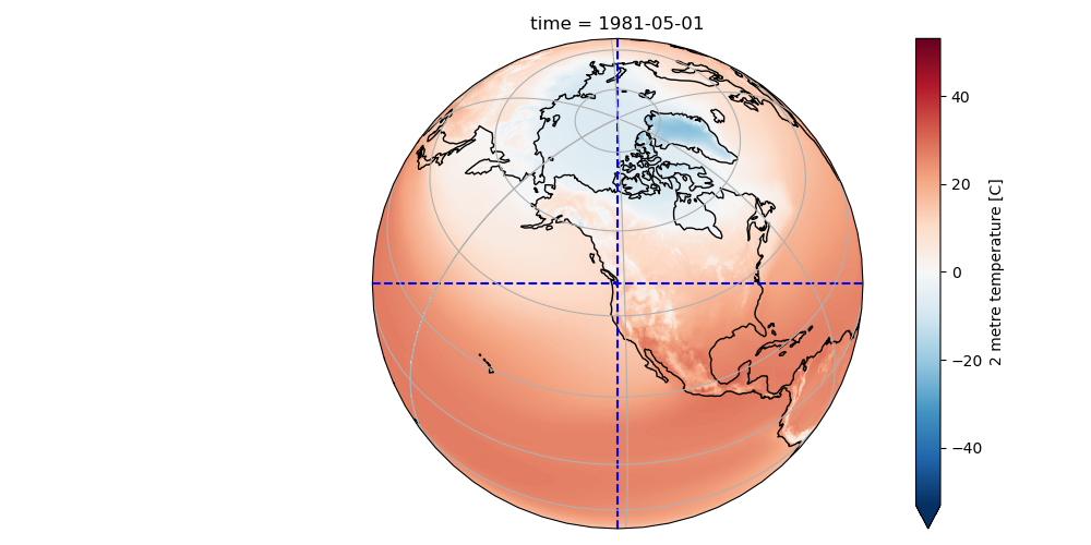
Create another cartopy plot for May, this time with an Orthographic projection centered on Seattle. Add dashed lines to indicate the center.#
# STUDENT CODE HERE
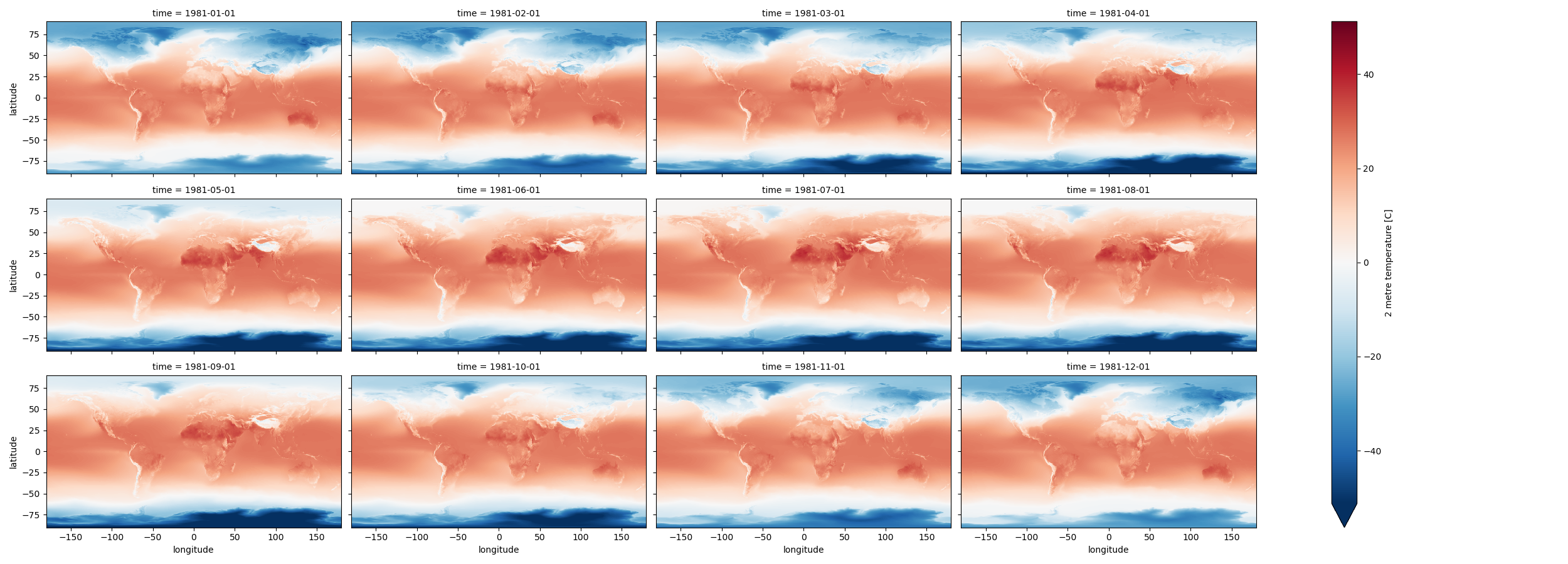
Create a Facet plot showing temperature grids for each month in the climatology Dataset#
http://xarray.pydata.org/en/stable/plotting.html#faceting
Note that these plots can be memory hungry, and if you have other kernels running, this could fill RAM and cause kernel to stop
Could try isolating a smaller area to test (see slicing) then running on full dataset when satisfied
Make sure your units are correct in the colorbar
Note that xarray uses a different definition of
aspectthan matplotlibhttps://docs.xarray.dev/en/stable/user-guide/plotting.html#controlling-the-figure-size
Since we have 360° of longitude and 180° of latitude, an aspect of 2 should work well here
While they may look similar, each panel is slightly different
Take a moment to admire this, look at seasonal cycles
# STUDENT CODE HERE
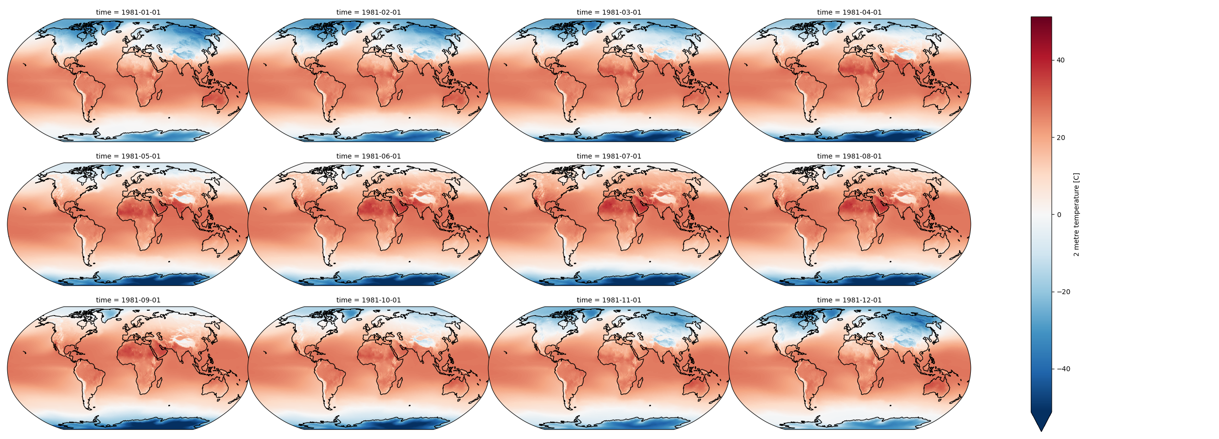
Now create a facetgrid plot in the Robinson projection and add coastlines#
Look at the second example in the xarray Maps documentation for inspiration
# STUDENT CODE HERE
Create an interactive plot with hvplot()#
Multiple plotting backends can be used with xarray
We previously used Seaborn, and folium/ipyleaflet for interactive maps
Still under development, but
hvplotis flexible and powerful:https://holoviz.org/
Note how coordinates and values are interactively displayed as you move your cursor over the plot
Experiment with time slider on right side
Experiment with zoom/pan capability
#clim_ds['t2m'].hvplot(x='longitude',y='latitude', cmap='RdBu_r', clim=(-50,50))
Written response: Using the interactive plot, what is the average 2 meter air temperature for Seattle in December?#
STUDENT WRITTEN RESPONSE HERE
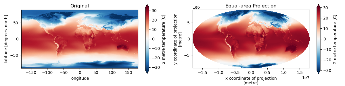
Reprojecting with rioxarray#
Those visualizations are nice, especially with cartopy when we can specify the projection of the axes. However, this is just for visualization, the actual dataset hasn’t been reprojected. This will be a problem for further analysis…
The netcdf files have equally spaced grid points every 0.25° of latitude and longitude, which means we are oversampling in the polar regions
Think back to Lab04 about the true distance covered by 0.25° degree of longitude near the pole (close to 0 m) vs 0.25° of longitude near the equator (~28 km)
The default Plate Carrée “projection” (cylindrical equidistant) for lat/lon data is fine for quick visualization, but it distorts area, especially in the polar regions
If we compute mean or other statistics without accounting for this, our results will be biased, incorrectly weigthing the polar regions
Fortunately, we can use
rioxarrayto quickly reproject into an equal-area projection for these calculationsFirst need to assigning a crs to the xarray dataset
Can then use
xds.rio.reproject()https://corteva.github.io/rioxarray/stable/examples/reproject.html
Caveat: The better way to do this would be to use the original Gaussian grid from the model, but since we have the netCDF data on regular grid, let’s just work with those
#Set CRS of the original xarray Datasets
clim_ds.rio.write_crs('EPSG:4326', inplace=True);
anom_ds.rio.write_crs('EPSG:4326', inplace=True);
print(clim_ds.spatial_ref)
<xarray.DataArray 'spatial_ref' ()> Size: 8B
array(0)
Coordinates:
    spatial_ref  int64 8B 0
Attributes:
    crs_wkt:                      GEOGCS["WGS 84",DATUM["WGS_1984",SPHEROID["...
    semi_major_axis:              6378137.0
    semi_minor_axis:              6356752.314245179
    inverse_flattening:           298.257223563
    reference_ellipsoid_name:     WGS 84
    longitude_of_prime_meridian:  0.0
    prime_meridian_name:          Greenwich
    geographic_crs_name:          WGS 84
    horizontal_datum_name:        World Geodetic System 1984
    grid_mapping_name:            latitude_longitude
    spatial_ref:                  GEOGCS["WGS 84",DATUM["WGS_1984",SPHEROID["...
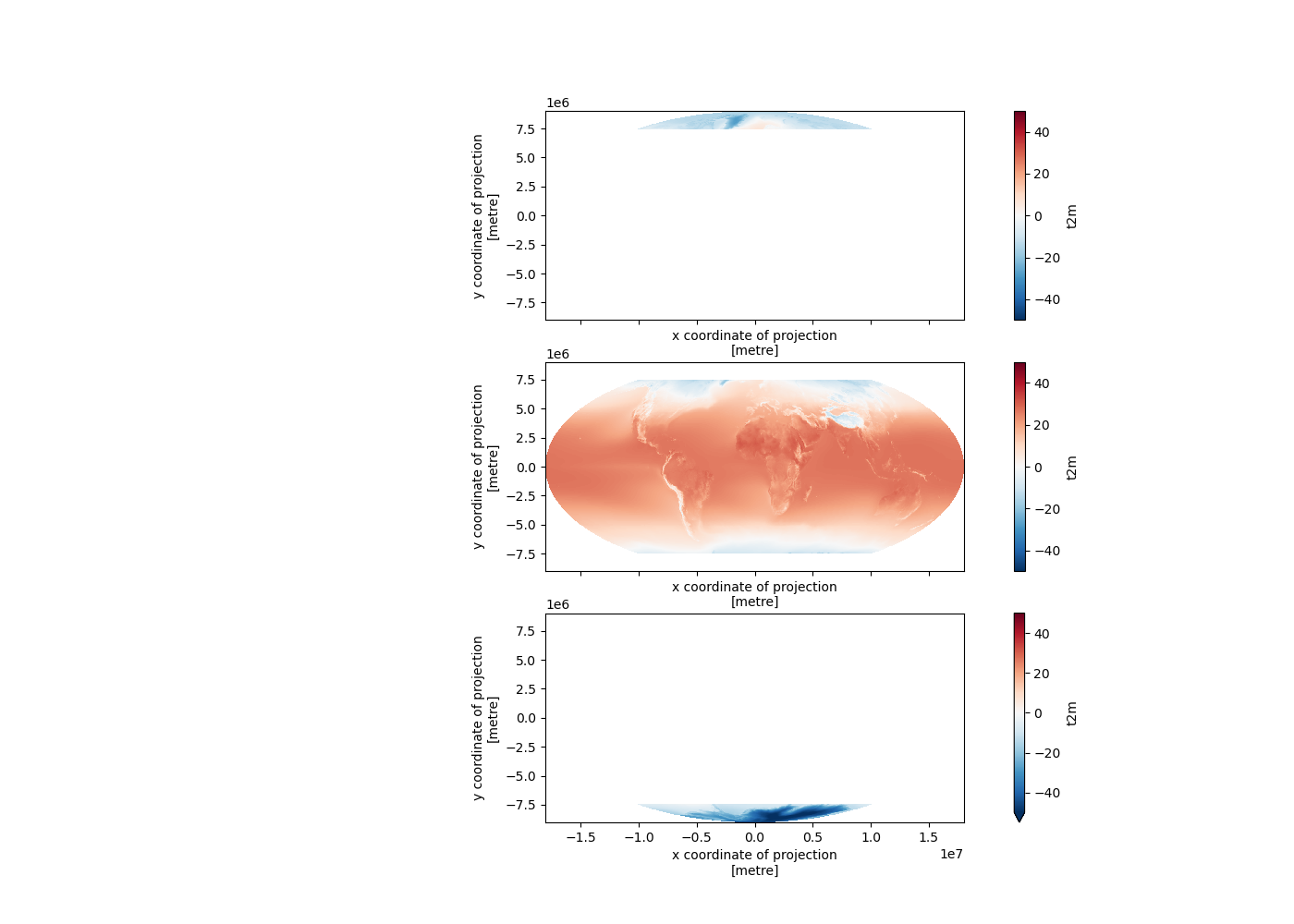
Reproject to the Mollweide projection using rioxarray. For January, plot the lat/lon data next to the reprojected Mollweide data.#
#Cylindrical equal area
ea_proj = '+proj=cea +lat_ts=45'
#Equal Earth (not working correctly)
ea_proj = '+proj=eqearth'
#Mollweide
ea_proj = '+proj=moll'
#ea_proj = 'EPSG:6933'
# STUDENT CODE HERE
# STUDENT CODE HERE
For both projections, compare the global mean temperature values for January, July, and the entire year.#
# STUDENT CODE HERE
Global mean temperature for January calculated in lat/lon: 3.53C
Global mean temperature for January calculated in equal-area projection: 12.25C
# STUDENT CODE HERE
Global mean temperature for July calculated in lat/lon: 7.78C
Global mean temperature for July calculated in equal-area projection: 16.06C
# STUDENT CODE HERE
Global mean temperature for the entire year calculated in lat/lon: 5.21C
Global mean temperature for the entire year calculated in equal-area projection: 14.18C
Much closer to expected value of 13.9° for 20th Century (https://www.ncei.noaa.gov/access/monitoring/monthly-report/global/)
Remember that our dataset is for 1979-2022 period, so we actually expect it to be slightly warmer than the average for the 1900-2000 period
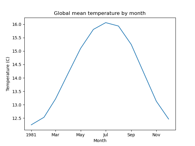
Create line plot of global monthly temperature#
Compute the mean of the reprojected climatology t2m DataArray across the spatial dimensions (both x and y)
Remember to pass the appropriate
dim=(...)tomean()so xarray knows over which dimensions to compute the mean!)
#Not this! Gives a single value for full array
#clim_da.mean()
# STUDENT CODE HERE
Create 2D plot showing mean temperature vs. latitude (averaged over all longitudes)#
# STUDENT CODE HERE

Written response: Based on your plot, which latitudes experience the “strongest seasons”?#
STUDENT WRITTEN RESPONSE HERE
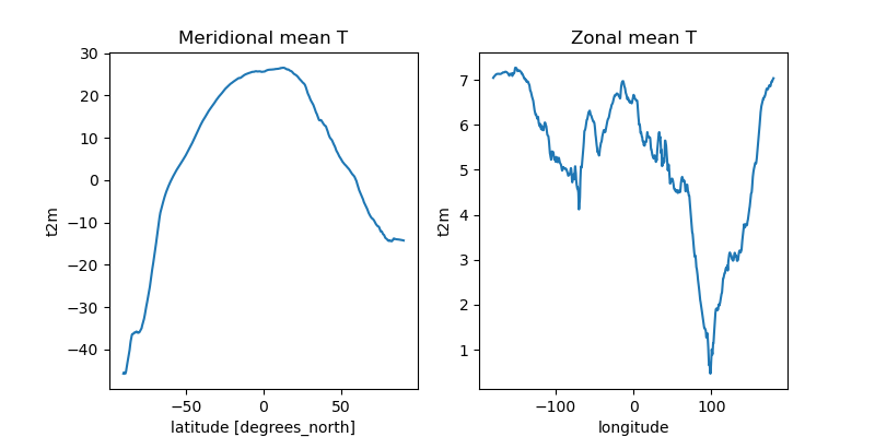
Create line plots of mean zonal and meridional temperature#
https://en.wikipedia.org/wiki/Zonal_and_meridional
Hint: specify a tuple of appropriate dimensions for the
dimkeyword when computingmean()Above we used
dim=('latitude', 'longitude')/dim=('x', 'y')to average all latitudes and longitudes / x and y values, plotting the resulting values over timeNow in the zonal mean case, we want to average for all latitudes and times, plotting resulting values vs. longitude
Create as figure with two subplots: meridional mean T and zonal mean T
Add titles accordingly
# STUDENT CODE HERE
Create a plot showing monthly mean temperature for the Arctic and Antarctic#
See location indexing here: http://xarray.pydata.org/en/stable/indexing.html#assigning-values-with-indexing
One approach:
Create boolean index arrays for
clim_ds['latitude']coordinate for relevant latitude rangesUse Arctic circle and Antarctic circle as a threshold
https://en.wikipedia.org/wiki/Arctic_Circle
Use the index array with xarray
wheremethod on theclim_ds['t2m']DataArrayMake sure to use
drop=Trueto avoid unnecessarily storing lots of nan values in memory
Compute the mean across all returned lat/lon grid cells
Note the magnitude and phase of the seasonal temperature varability at the opposite poles
polar_lat = 66.5 #degrees
Convert polar circle latitude to y-coordinate for equal area projection#
#Compute y coordinate of polar circle latitude
from pyproj import CRS, Transformer
transformer = Transformer.from_crs(CRS.from_epsg(4326), CRS.from_proj4(ea_proj))
polar_y = transformer.transform(polar_lat, 0)[-1]
polar_y
7474236.788842151
arctic_idx = (clim_da['y'] >= polar_y)
antarctic_idx = (clim_da['y'] <= -polar_y)
nonpolar_idx = (clim_da['y'] < polar_y) & (clim_da['y'] > -polar_y)
#Confidence check
#arctic_idx[::10]
#antarctic_idx[::10]
#nonpolar_idx[::10]
kwargs = dict(cmap='RdBu_r', vmin=-50, vmax=50)
Plot the global mean temperature, with seperate plots for the three regions (arctic, non-polar, antarctic)#
# STUDENT CODE HERE
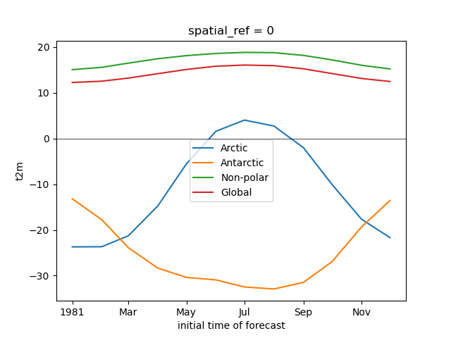
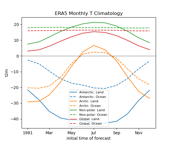
Plot the average temperature for each month for the entire globe, arctic, antarctic, and non-polar seperately#
# STUDENT CODE HERE
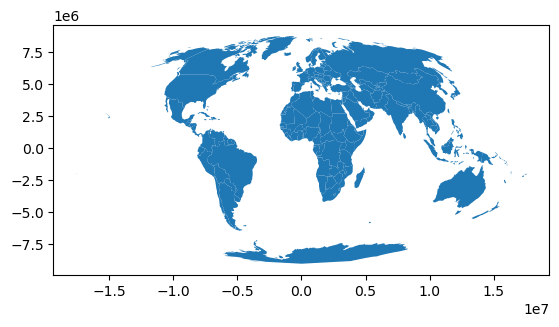
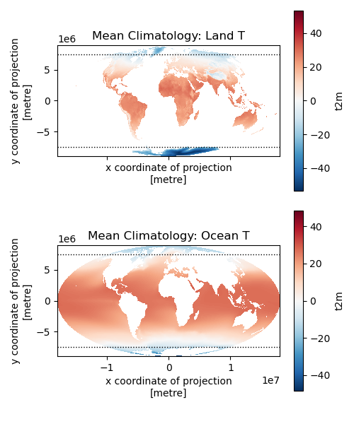
Challenge question: Repeat the above analysis, isolating land and ocean classes (GS: Attempt required / UG: +1 pts)#
Hint: can use
rioxarrayfor clipping using a GeoDataFrame or geometry, perhaps using the world polygons we’ve used before
world = gpd.read_file("https://naciscdn.org/naturalearth/110m/cultural/ne_110m_admin_0_countries.zip")
world = world.to_crs(ea_proj)
world.plot();
# STUDENT CODE HERE
# STUDENT CODE HERE
# STUDENT CODE HERE
# STUDENT CODE HERE
Written response: Describe some insights from splitting each zone into its land and ocean components#
STUDENT WRITTEN RESPONSE HERE
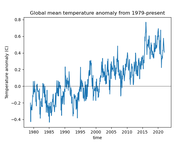
Part 2: Global temperature variability from 1979-present (6 pts)#
Can we see evidence of climate change in reanalysis datasets? Let’s check.
To do this, we will use the monthly anomalies from 1979-present, contained in the anom_ds Dataset
#Reproject anomaly dataset to equal area projection
#This temporarily requires ~6 GB RAM
anom_da = anom_ds['t2m'].rio.reproject(ea_proj)
Create a line plot of mean global monthly temperature anomaly from 1979-present#
Note: if you used xarray’s default lazy load of the
ncfile, and this is the first time reading the entireanom_dsfrom disk, this may take ~20 seconds
# STUDENT CODE HERE
# STUDENT CODE HERE
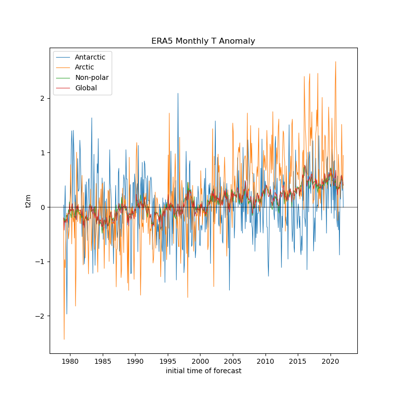
Did the Arctic and Antarctic warm at the same rate over the past 40 years?#
Create a line plot showing anomalies for each region, you can reuse indices from above
# STUDENT CODE HERE
# STUDENT CODE HERE
# STUDENT CODE HERE
# STUDENT CODE HERE
Compute linear temperature trend at each pixel and create a map with coastlines#
Note: can coarsen the data to 1x1° to improve performance (16x!)
See the xarray
polyfitfunction: https://docs.xarray.dev/en/stable/generated/xarray.DataArray.polyfit.htmlA linear fit is degree 1
This will return two coefficients (m and b in y=mx+b), so we want to consider m here
anom_ds.dims
FrozenMappingWarningOnValuesAccess({'time': 517, 'latitude': 721, 'longitude': 1440})
ds_factor=4
anom_ds_1deg = anom_ds.coarsen(latitude=ds_factor, longitude=ds_factor, boundary='trim').mean()
anom_ds_1deg.dims
FrozenMappingWarningOnValuesAccess({'time': 517, 'latitude': 180, 'longitude': 360})
#The difference along the time axis will return values in degrees C per timedelta64[ns] - nanoseconds
#We want degrees C per year
#Conversion factor from nanoseconds to year
dt_factor = 1E9 * (60*60*24*365.25)
# STUDENT CODE HERE
# STUDENT CODE HERE
years = pd.DatetimeIndex(anom_ds_1deg.time.values).year
# STUDENT CODE HERE
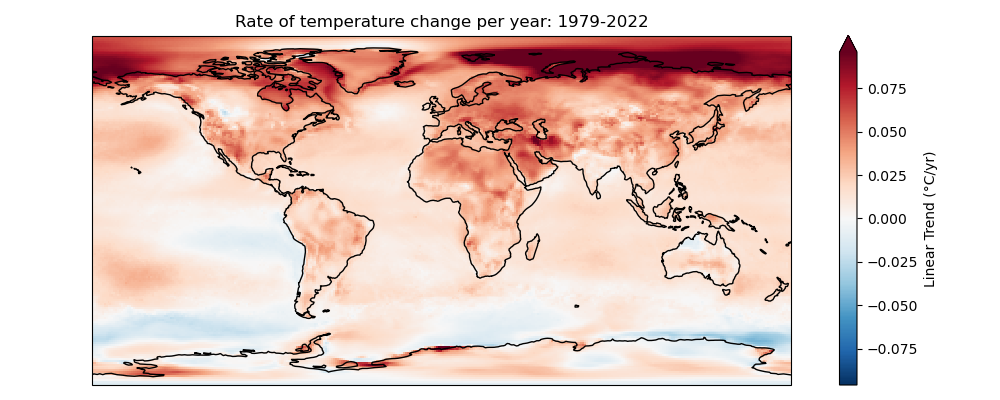
Written response: From 1979 to 2022, what general trends do you see? Where is warming greatest? Where is cooling greatest? Why might you prefer this plot over the global line plot?#
STUDENT WRITTEN RESPONSE HERE
Part 3: Analyze WA snow depth with ERA5 Land daily data (7 pts)#
Now we’ll look at the ERA5 Land product, which is a higher resolution 9km dataset. We’ll use the daily averages of the temperature and snow depth variables hosted on Google Earth Engine, and we’ll pull them down dynamically from Google Earth Engine using the Google Earth Engine Python API and Xee. We will focus on water year 2021.
Get the WA state outline#
states_url = 'http://eric.clst.org/assets/wiki/uploads/Stuff/gz_2010_us_040_00_500k.json'
states_gdf = gpd.read_file(states_url)
wa_state_gdf = states_gdf.loc[states_gdf['NAME'] == 'Washington']
wa_state_gdf
| GEO_ID | STATE | NAME | LSAD | CENSUSAREA | geometry | |
|---|---|---|---|---|---|---|
| 14 | 0400000US53 | 53 | Washington | 66455.521 | MULTIPOLYGON (((-123.09055 49.00198, -123.0353... |
We’ll use this helper function to abstract away most of the data download complexities#
def get_era5_land_daily(
    bbox_gdf: gpd.GeoDataFrame | None = None,
    start_date: str | None = None,
    end_date: str | None = None,
    variables: str | list | None = None,
) -> xr.Dataset:
    """
    ERA5-Land reanalysis data for a given bounding box and time period.

    Description:
    ERA5 is the fifth generation ECMWF atmospheric reanalysis of the global climate.
    ERA5 provides hourly estimates of many atmospheric, land-surface and sea-state parameters.

    Parameters
    ----------
    bbox_gdf : geopandas.GeoDataFrame or tuple or shapely.Geometry, optional
        GeoDataFrame containing the bounding box, or a tuple of (xmin, ymin, xmax, ymax), or a Shapely geometry.
    start_date : str, optional
        Start date in 'YYYY-MM-DD' format. If None, uses earliest available date.
    end_date : str, optional
        End date in 'YYYY-MM-DD' format. If None, uses latest available date.
    variables : str or list, optional
        Variable(s) to select. If None, returns all variables.


    Returns
    -------
    xarray.Dataset
        ERA5 dataset with selected variables and dimensions.

    Examples
    --------
    >>> import easysnowdata
    >>>
    >>> # Get monthly ERA5 temperature data for a region
    >>> bbox = (-122.5, 47.0, -121.5, 48.0)
    >>> era5_ds = easysnowdata.remote_sensing.get_era5(
    ...     bbox,
    ...     start_date='2020-01-01',
    ...     end_date='2020-12-31',
    ...     variables=['temperature_2m']
    ... )

    Notes
    -----
    Data citation:
    Hersbach, H., Bell, B., Berrisford, P., et al. (2020). The ERA5 global reanalysis.
    Quarterly Journal of the Royal Meteorological Society, 146(730), 1999-2049.
    """
    service_account = 'gdawinter2025@gda-winter25.iam.gserviceaccount.com'
    credentials = ee.ServiceAccountCredentials(service_account, 'private_key.json')
    ee.Initialize(credentials, opt_url='https://earthengine-highvolume.googleapis.com')

    collection_name = "ECMWF/ERA5_LAND/DAILY_AGGR"

    # Initialize image collection
    image_collection = ee.ImageCollection(collection_name)

    # Apply date filtering if specified
    if start_date is not None and end_date is not None:
        image_collection = image_collection.filterDate(start_date, end_date)

    # Apply variable selection if specified
    if variables is not None:
        if isinstance(variables, str):
            variables = [variables]
        image_collection = image_collection.select(variables)

    # Get projection from first image
    image = image_collection.first()
    projection = image.select(0).projection()

    # Convert bbox if provided
    geometry = tuple(bbox_gdf.total_bounds)

    # Load dataset
    ds = xr.open_dataset(
        image_collection,
        engine='ee',
        geometry=geometry,
        projection=projection,
        chunks=None
    )

    # Clean up dimensions and coordinate names
    ds = (ds
          .transpose('time', 'lat', 'lon')
          .rename({'lat': 'latitude', 'lon': 'longitude'})
          .rio.set_spatial_dims(x_dim='longitude', y_dim='latitude'))

    # Add metadata
    ds.attrs['data_citation'] = "Hersbach, H., Bell, B., Berrisford, P., et al. (2020). The ERA5 global reanalysis. Quarterly Journal of the Royal Meteorological Society, 146(730), 1999-2049."

    return ds
wa_era5_ds = get_era5_land_daily(bbox_gdf=wa_state_gdf, start_date='2020-10-01', end_date='2021-10-01', variables=['temperature_2m','snow_depth'])
wa_era5_ds
<xarray.Dataset> Size: 8MB
Dimensions:         (time: 365, longitude: 78, latitude: 35)
Coordinates:
  * time            (time) datetime64[ns] 3kB 2020-10-01 ... 2021-09-30
  * longitude       (longitude) float64 624B -124.7 -124.6 ... -117.1 -117.0
  * latitude        (latitude) float64 280B 48.95 48.85 48.75 ... 45.65 45.55
Data variables:
    temperature_2m  (time, latitude, longitude) float32 4MB ...
    snow_depth      (time, latitude, longitude) float32 4MB ...
Attributes:
    crs:            EPSG:4326
data_citation: Hersbach, H., Bell, B., Berrisford, P., et al. (2020). Th...Use the following Albers Equal Area projection for WA state to reproject the WA state geodataframe and reproject the ERA5 dataset. Then clip the dataset by the WA geometry#
In the
.rio.clip()call, pass indrop=True
wa_crs = "+proj=aea +lon_0=-120.8496094 +lat_1=45.79505 +lat_2=48.6191076 +lat_0=47.2070788 +datum=WGS84 +units=m +no_defs"
# STUDENT CODE HERE
# STUDENT CODE HERE
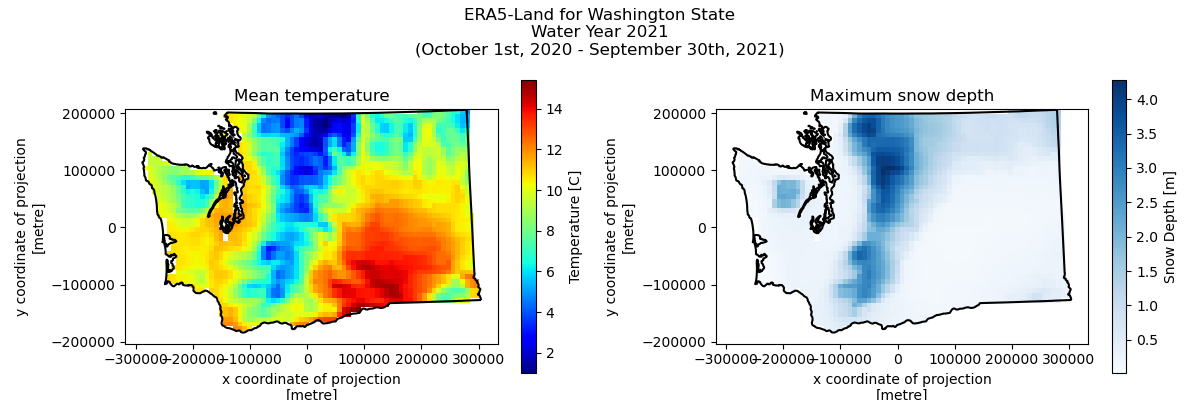
Convert the temperature variable to C. Then plot the average temperature and maximum snow depth.#
# STUDENT CODE HERE
# STUDENT CODE HERE
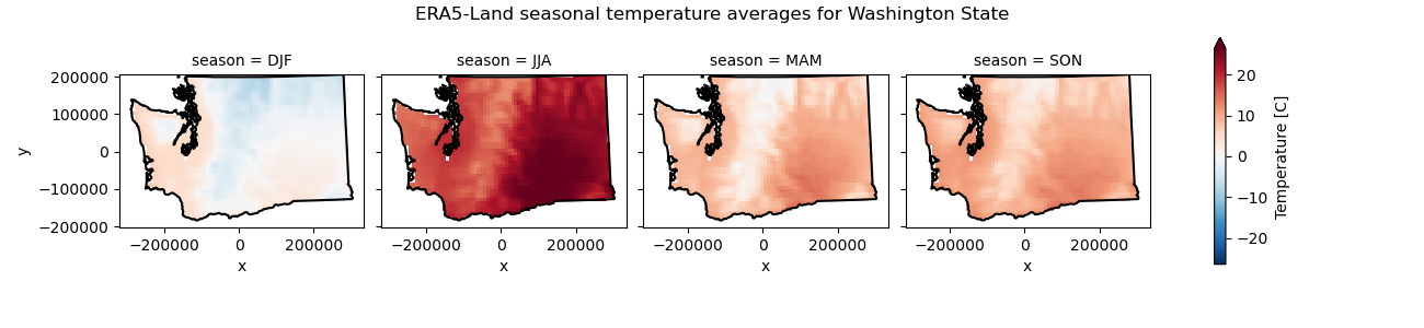
Compute seasonal temperature averages and then show these on a facetgrid plot#
# STUDENT CODE HERE
Compute monthly snow depth averages, and then show these on a facetgrid plot#
You could do
.groupby("time.month"), but try.resample(time='ME')instead
# STUDENT CODE HERE

Written response: Do these mean temperatures seem reasonable? What is the greatest max snow depth you see? Do you think this is truly the greatest maximum snow depth for water year 2021 in Washington? Why?#
STUDENT WRITTEN RESPONSE HERE
Create a line plot of state-wide temperature and snow depth averages over time#
# STUDENT CODE HERE
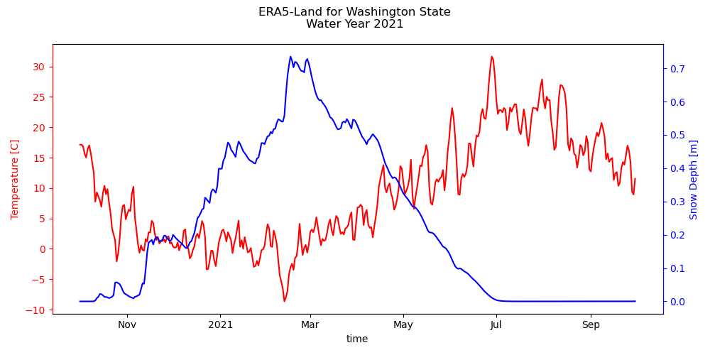
Calculate the minimum average state-wide temperature and maximum state-wide snow depth and when they occured respectively#
Hint: try using
.idxmin()and.idxmax()to get a datetime object, and then.dt.strftime('%Y-%m-%d').valuesto convert it to a string
# STUDENT CODE HERE
The minimum average state-wide temperature was -8.64C, occuring on 2021-02-12
The maximum average state-wide snow depth was 0.74m, occuring on 2021-02-16
Written response: Do these timings make sense? Where do you think the maximum statewide snow depth occured? Generally, where does snow persist the longest, and why?#
STUDENT WRITTEN RESPONSE HERE
We’ve provided you with a snow depth time-series as measured by an automatic weather station near Mt. Rainier. For water year 2021, create a plot with the station’s snow depth time series and the ERA5-Land snow depth of the pixel that contains the weather station.#
Hint: You’ll have to take the lat / lon values from the dataarray and convert them to the projected coordinate system!
import easysnowdata
AllStations = easysnowdata.automatic_weather_stations.StationCollection()
AllStations.get_entire_data_archive()
Geodataframe with all stations has been added to the Station object. Please use the .all_stations attribute to access.
Use the .get_data(stations=geodataframe/string/list,variables=string/list,start_date=str,end_date=str) method to fetch data for specific stations and variables.
Downloading compressed data to a temporary directory (/tmp/all_station_data.tar.lzma)...
Decompressing data...
Creating xarray.Dataset from the uncompressed data...
Done! Entire archive dataset has been added to the station object. Please use the .entire_data_archive attribute to access.
snotel_da = AllStations.entire_data_archive["SNWD"]
snotel_da = snotel_da[snotel_da['state']=='Washington']
station_da = snotel_da.sel(station="679_WA_SNTL")
station_da
<xarray.DataArray 'SNWD' (time: 24164)> Size: 193kB
array([   nan,    nan,    nan, ..., 3.0226, 3.175 , 3.429 ])
Coordinates: (12/17)
  * time           (time) datetime64[ns] 193kB 1909-04-13 ... 2025-02-18
    station        <U12 48B '679_WA_SNTL'
    name           <U24 96B 'Paradise'
    network        <U6 24B 'SNOTEL'
    elevation_m    float64 8B 1.564e+03
    latitude       float64 8B 46.78
    ...             ...
    beginDate      datetime64[ns] 8B 1979-10-01
    endDate        datetime64[ns] 8B 2025-02-27
    csvData        bool 1B True
    geometry       object 8B POINT (-121.74765014648438 46.782649993896484)
    WY             (time) int64 193kB 1909 1955 1955 1955 ... 2025 2025 2025
DOWY (time) int64 193kB 195 62 63 64 65 66 ... 137 138 139 140 141# STUDENT CODE HERE
(-68557.62942671867, -46803.71791344562)
# STUDENT CODE HERE
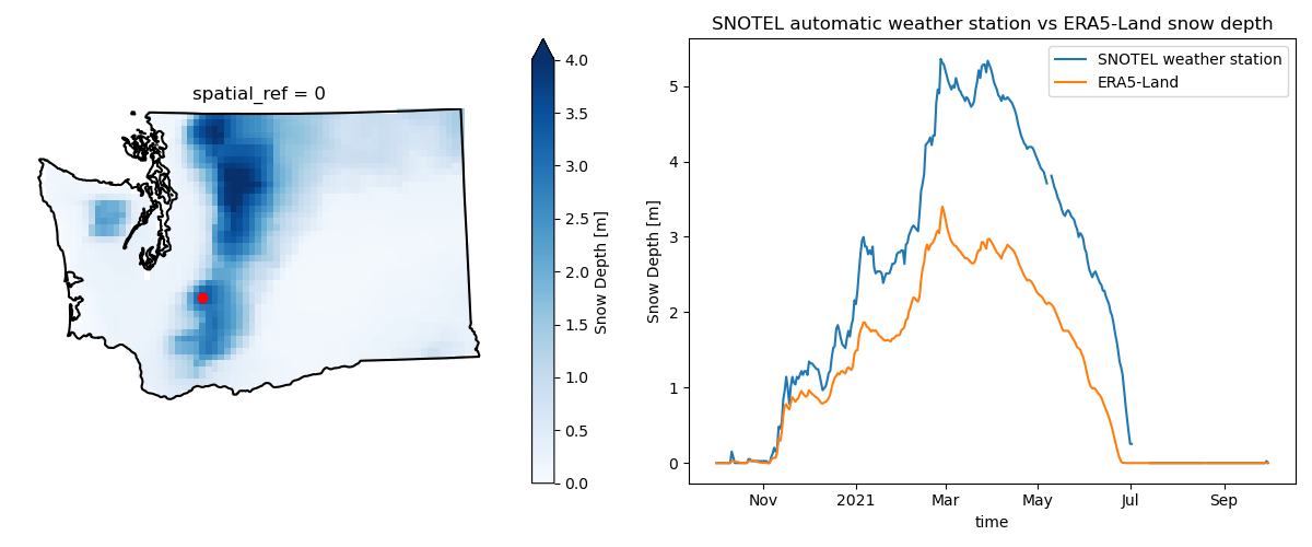
Written response: For the two snow depth time-series, comment on differences or similarities in trends, magnitude, and timing. Give some reasons for why there might be differences between the two time-series.#
STUDENT WRITTEN RESPONSE HERE
Submission#
Save the completed notebook (make sure to fully run the notebook and check all cell output is visible)
Use the
git add; git commit -m 'message'; git pushworkflow to push your work to the remote repositoryideally you’ve been using add / commit / push as you make progress on this notebook
Check the remote repository to check all of the files you want to submit have been pushed
Scroll through your jupyter notebook on your remote repository and make sure all output and plots are visible
When you have completed your last push, submit the url pointing to your Github repository to the corresponding Canvas assignment